Surface Fitting and Smoothing
Surface Smoothing
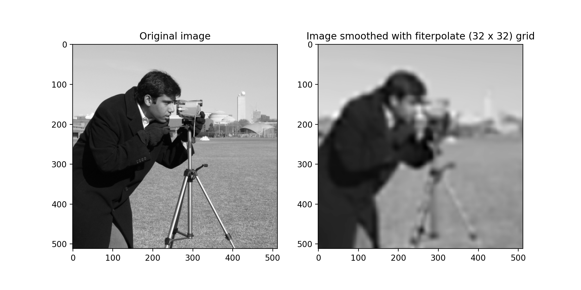
The surface fitting procedures replicate some of the numerical functions from
the IDL fspextool package. fiterpolate() is the wrapper for
many of these functions, designed to fit cubic polynomials to subsections of
an image, derive values and derivates at the intersections, then apply
bicubic interpolation to create a smoothed image. In general, the
sofia_redux.toolkit.resampling or sofia_redux.toolkit.convole modules are better
suited to image smoothing, and can also deal with data in N-dimensions.
fiterpolate() must be supplied with the number of rows and columns with
which to create a regular grid on which to calculate values and derivatives
prior to interpolation.
from sofia_redux.toolkit.image.smooth import fiterpolate
import matplotlib.pyplot as plt
import imageio

image = imageio.imread('imageio:camera.png').astype(float)
image -= image.min()
image /= image.max()

smoothed = fiterpolate(image, 32, 32)
fig, ax = plt.subplots(nrows=1, ncols=2, figsize=(10, 5))
ax[0].imshow(image, cmap='gray')
ax[0].set_title("Original image")
ax[1].imshow(smoothed, cmap='gray')
ax[1].set_title("Image smoothed with fiterpolate (32 x 32) grid")
(Source code, png, hires.png, pdf)

Surface Coefficients
The quadfit() function is used by fiterpolate() to generate
the coefficients necessary for subsequent bicubic evaluation. Essentially,
it uses a stripped down version of
sofia_redux.toolkit.fitting.polynomial.polyfit() to calculate the coefficients
(\(c\)) for the following function:
\[f(x, y) = c_{0,0} + c_{1, 0}x + c_{0, 1}y + c_{2, 0}x^2 + c_{0, 2}y^2 + c_{1, 1}xy\]
For example,
import numpy as np
from sofia_redux.toolkit.image.smooth import quadfit

y, x = np.mgrid[:5, :5]
z = 1 + (2 * x) + (3 * y) + (4 * x ** 2) + (5 * y ** 2) + (6 * x * y)
coefficients = quadfit(z)
coefficients
Output:
array([1., 2., 3., 4., 5., 6.])
As can be seen, this is very basic since no dependent variables can be
specified and the input array must be an image. Therefore, for anything
more advanced than this, sofia_redux.toolkit.fitting.polynomial.polyfit() should
be used.
Bi-Cubic Coefficients and Evaluation
bicubic_coefficients() and bicubic_evaluate() are used to create
a surface fit using the values, derivatives, and cross derivate at the 4
vertices of a square. The vertices must be provided in the order: lower-left,
upper-left, upper-right, lower-right. Coefficients are evaluated by applying
the following weights matrix:
\[\begin{split}W = \begin{bmatrix} 1 & 0 & 0 & 0 & 0 & 0 & 0 & 0 & 0 & 0 & 0 & 0 & 0 & 0 & 0 & 0 \\ 0 & 0 & 0 & 0 & 0 & 0 & 0 & 0 & 1 & 0 & 0 & 0 & 0 & 0 & 0 & 0 \\ -3 & 0 & 0 & 3 & 0 & 0 & 0 & 0 & -2 & 0 & 0 & -1 & 0 & 0 & 0 & 0 \\ 2 & 0 & 0 & -2 & 0 & 0 & 0 & 0 & 1 & 0 & 0 & 1 & 0 & 0 & 0 & 0 \\ 0 & 0 & 0 & 0 & 1 & 0 & 0 & 0 & 0 & 0 & 0 & 0 & 0 & 0 & 0 & 0 \\ 0 & 0 & 0 & 0 & 0 & 0 & 0 & 0 & 0 & 0 & 0 & 0 & 1 & 0 & 0 & 0 \\ 0 & 0 & 0 & 0 & -3 & 0 & 0 & 3 & 0 & 0 & 0 & 0 & -2 & 0 & 0 & -1 \\ 0 & 0 & 0 & 0 & 2 & 0 & 0 & -2 & 0 & 0 & 0 & 0 & 1 & 0 & 0 & 1 \\ -3 & 3 & 0 & 0 & -2 & -1 & 0 & 0 & 0 & 0 & 0 & 0 & 0 & 0 & 0 & 0 \\ 0 & 0 & 0 & 0 & 0 & 0 & 0 & 0 & -3 & 3 & 0 & 0 & -2 & -1 & 0 & 0 \\ 9 & -9 & 9 & -9 & 6 & 3 & -3 & -6 & 6 & -6 & -3 & 3 & 4 & 2 & 1 & 2 \\ -6 & 6 & -6 & 6 & -4 & -2 & 2 & 4 & -3 & 3 & 3 & -3 & -2 & -1 & -1 & -2 \\ 2 & -2 & 0 & 0 & 1 & 1 & 0 & 0 & 0 & 0 & 0 & 0 & 0 & 0 & 0 & 0 \\ 0 & 0 & 0 & 0 & 0 & 0 & 0 & 0 & 2 & -2 & 0 & 0 & 1 & 1 & 0 & 0 \\ -6 & 6 & -6 & 6 & -3 & -3 & 3 & 3 & -4 & 4 & 2 & -2 & -2 & -2 & -1 & -1 \\ 4 & -4 & 4 & -4 & 2 & 2 & -2 & -2 & 2 & -2 & -2 & 2 & 1 & 1 & 1 & 1 \\ \end{bmatrix}\end{split}\]
to the following values:
\[A = \begin{bmatrix} f(ll) & f(ul) & f(ur) & f(lr) & \frac{\partial f}{\partial x}(ll) \dots & \frac{\partial f}{\partial y}(ll) \dots & \frac{\partial^2 f}{\partial x y}(ll) \dots & \frac{\partial^2 f}{\partial x y}(ur) \end{bmatrix}\]
where \(ll\) indicates the lower-left vertex and \(ur\) indicates the upper right vertex. The final cubic coefficients (\(C\)) are then given by
\[C^{\prime} = W A\]
We then reshape the matrix such that
\[vec(C) = C^{\prime} \, | \, C \in \mathbf{R}^{4, 4}\]
or in python:
c_prime = (W @ A).reshape(4, 4)
To evaluate these cubic coefficients over the unit square, where \((x, y) = (0, 0)\) is the lower-left coordinate and \((1, 1)\) is the upper-right coordinate:
\[f(x, y) = \sum_{i=0}^{3} \sum_{j=0}^{3} {c_{i,j} x^i y^j}\]
A more detailed numerical analysis can be found in section 3.6 of Numerical
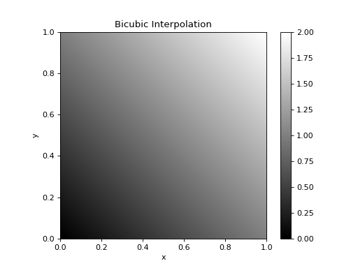
Recipes in C. bicubic_evaluate() calls bicubic_coefficients()
to evaluate the fit at new (x, y) coordinates. As a quick example, here is
bicubic_evaluate() on f(x, y) = x + y:
import numpy as np
import matplotlib.pyplot as plt
from sofia_redux.toolkit.image.smooth import bicubic_evaluate

z_corners = np.array([0.0, 1.0, 2.0, 1.0])  # values at corners
dx = np.full(4, 1.0)  # x-gradients at corners
dy = dx.copy()  # y-gradients at corners
dxy = np.zeros(4)  # not present here
xrange = [0, 1]
yrange = [0, 1]

x, y = np.meshgrid(np.linspace(0, 1, 100), np.linspace(0, 1, 100))
z_new = bicubic_evaluate(z_corners, dx, dy, dxy, xrange, yrange, x, y)
plt.imshow(z_new, origin='lower', cmap='gray', extent=[0, 1, 0, 1])
plt.colorbar()
plt.title("Bicubic Interpolation")
plt.xlabel("x")
plt.ylabel("y")
(Source code, png, hires.png, pdf)

The sofia_redux.toolkit.fitting module contains many more powerful fitting
functions that could be applied here instead.
sofia_redux.toolkit.image.fiterpolate was created to replicate the fiterpolate
algorithm originally developed in the 1980’s by J. Tonry, and exists to
support any algorithm that may require a Python implementation.