Mask and NaN Image Filling

There are two different algorithms for filling holes in an image. Holes are defined by either a 2-D array mask of bool values, the same shape as the image, in which False indicates a hole or bad value, and True indicates a value that is valid. The alternative is to use NaN values in the image itself to identify holes in the image that should be filled in.

Aside from the functions mentioned here, the sofia_redux.toolkit.convolve module contains classes and functions that would perform similarly. However, the user would have to select the correct kernel for their purposes and ensure it is sufficiently large enough to cover the largest hole.

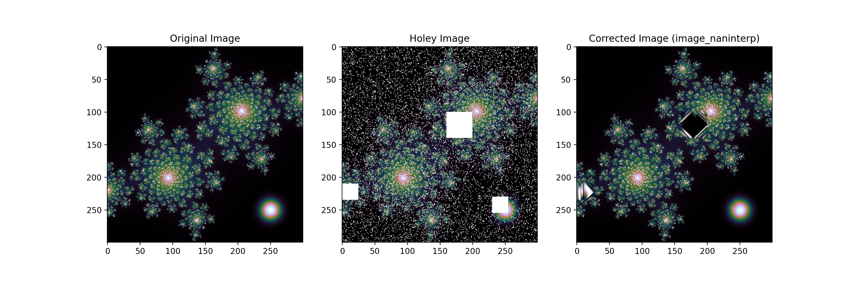
2-D Clough-Tocher Interpolation (image_naninterp())

image_naninterp() implements the Clough-Tocher scheme which first creates a triangulation of the available (non-masked/finite) data values in the image. For a single triangle, a 12 term cubic polynomial is created consisting of the value and derivatives at each vertex (\(f, f_x^\prime, f_y^\prime\)) and the cross-boundary derivatives (\(\partial f / \partial n\)) at the edge midpoints.

The final result can be evaluated fairly quickly as a piecewise polynomial, \(C^1\) surface with quadratic precision. Unfortunately, since this is only generated for the convex hull of points, extrapolation beyond the convex hull is not possible. Therefore, if a hole exist at the edge of the image, it may not be able to be filled using this method, or the same interpolation rules cannot be guaranteed.

import numpy as np
import matplotlib.pyplot as plt
from sofia_redux.toolkit.image.fill import image_naninterp
from sofia_redux.toolkit.utilities.func import julia_fractal
from astropy.modeling.models import Gaussian2D

image = julia_fractal(300, 300)
g = Gaussian2D(x_mean=250, y_mean=250, x_stddev=10, y_stddev=10)
image += g(*np.meshgrid(np.arange(300), np.arange(300)))
original = image.copy()

# add a few single pixel holes
rand = np.random.RandomState(41)
mask = rand.rand(*image.shape[:2]) < 0.1
image[mask] = np.nan

# add some larger holes
image[210:235, 0:25] = np.nan  # edge example
image[100:140, 160:200] = np.nan  # large structure example
image[230:255, 230:255] = np.nan  # smooth example
bad = image.copy()
image = np.clip(image_naninterp(image), 0, 1)

fig, ax = plt.subplots(nrows=1, ncols=3, figsize=(15, 5))
c = 'cubehelix' #'jet'
ax[0].imshow(original, cmap=c)
ax[0].set_title("Original Image")
ax[1].imshow(bad, cmap=c)
ax[1].set_title("Holey Image")
ax[2].imshow(image, cmap=c)
ax[2].set_title("Corrected Image (image_naninterp)")

(Source code, png, hires.png, pdf)

In the above example it can be seen that all small holes were filled fairly well, but the larger holes near the left and middle of the image show obviously incorrect structure, with severe striations near the edge. However, the smooth feature to the bottom-right was reconstructed nicely. Bear in mind that nan_interp() can only fit to quadratic precision, so the missing section of the Gaussian near the bottom-right was fit adequately, but it would be impossible to correct for fine structure over a large scale. Therefore, care should be taken when using nan_interp() on noisy images or when prominent small scale features are present.

Iterative Filling (maskinterp())

The maskinterp() function is a Python adaption of the IDL spextool function of the same name with added functionality. The function takes an image in which bad values are marked by either NaNs, or a supplied mask, but not both. Be careful if supplying a mask to an image containing NaNs where a mask value of True corresponds to a NaN value in the image.

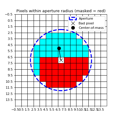
The algorithm works iteratively: Each bad pixel is corrected using the surrounding pixels within a circular aperture centered over the bad pixel. The function used for this task is up to the user (polynomial fit by default). There are three conditions that need to be met before a replacement value for the bad pixel is determined:

1. There are enough good (finite/unmasked) pixels within the aperture to perform a successful fit. For example, a 3rd order polynomial fit requires 16 pixels (4 in the x and y directions). The minimum number of points allowable is set by the minpoints parameter.

2. The bad pixel is within a certain distance from the center-of-mass of good pixels within the aperture. For example, this would stop extrapolation in the case where there were enough good pixels to theoretically perform a fit, but they were all to one side of the bad pixel. The default distance limit is 1 pixel and may be set with the cdis parameter.

3. The fraction of unmasked/finite pixels inside the aperture must be greater than minfrac (default=0.2).

(Source code, png, hires.png, pdf)

If a fit cannot be performed due to one of the above limitations, the aperture radius is increased by apstep pixels (default=1) and the procedure is repeated. Iteration is halted once all bad values have been filled or the aperture radius is greater than maxap. If a pixel cannot be filled, it is replaced with cval (NaN by default).

Example

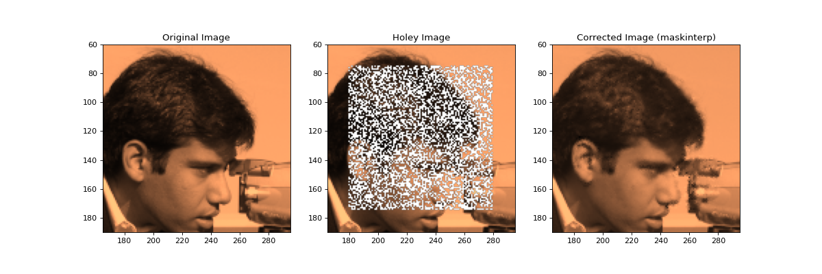
import matplotlib.pyplot as plt
import numpy as np
import imageio
from sofia_redux.toolkit.image.fill import maskinterp

image = imageio.imread('imageio:camera.png').astype(float)
image /= image.max()
original = image.copy()
rand = np.random.RandomState(41)
badpix = rand.rand(100, 100) > 0.5
cut = image[75:175, 180:280]
cut[badpix] = np.nan

result = maskinterp(image, kx=2, ky=2, minpoints=9)
fig, ax = plt.subplots(nrows=1, ncols=3, figsize=(15, 5))
c = 'copper'
ax[0].imshow(original, cmap=c)
ax[0].set_title("Original Image")
ax[1].imshow(image, cmap=c)
ax[1].set_title("Holey Image")
ax[2].imshow(result, cmap=c)
ax[2].set_title("Corrected Image (maskinterp)")
for a in ax:
    a.set_xlim(165, 295)
    a.set_ylim(190, 60)

(Source code, png, hires.png, pdf)

The above example fits a second order polynomial using the maskinterp algorithm. We require that a minimum of 9 points is used to fit good points (3 in X * 3 in Y).

Maskinterp Fitting Function

The fitting function can be set with the func parameter. There are two types of function available:

1. Statistical: fit = f(pixel_values, **kwargs)

2. Dependent: fit = f(pixel_values, cin, cout, **kwargs)

Statistical functions only require the pixel values within the aperture, while dependent functions require the input pixel coordinates and output pixel coordinates. For maskinterp() cin and cout must always be (N, 2) arrays where cin[:, 0] contains the y coordinates of the input pixels, and cin[:, 1] contains the x coordinates of the input pixels. i.e., create a fit based on the data values and cin, then interpolate onto any values contained in cout.

For example, the following function defines the default polynomial fitting function:

def spline_interp_2dfunc(d, cin, cout, **kwargs):
    return polyinterp2d(
        cin[:, 1], cin[:, 0], d, cout[:, 1], cout[:, 0], **kwargs)

A statistical function could be defined as shown in the following example:

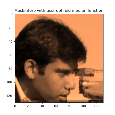
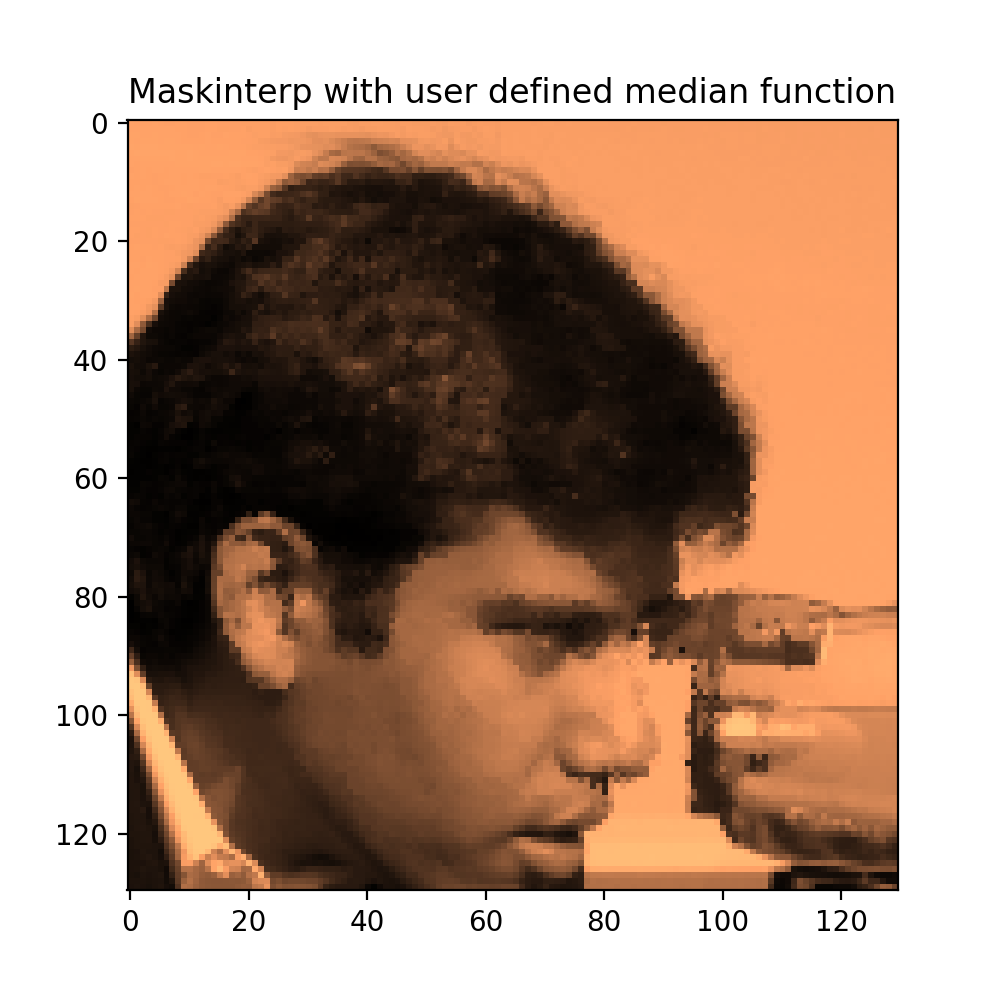
median_filled = maskinterp(image, func=np.median, statistical=True)
plt.figure(figsize=(5, 5))
plt.imshow(median_filled[60:190, 165:295], cmap='copper')
plt.title("Maskinterp with user defined median function")

(Source code, png, hires.png, pdf)

In order to declare that the function being used does not rely on input/output coordinates, statistical=True must be set.

Performance

The processing time required for maskinterp() is highly dependent on the number of masked points in an image, the scale of any holes (number of iterations), and the function used to fit. image_naninterp() is only dependent on the size of the image. Therefore, if performance is a consideration, testing is required. Otherwise, the sofia_redux.toolkit.convolve module also allows replacement of masked/NaN values through convolution of valid points with a given kernel including a Savitzky-Golay polynomial approximation.

Polygon Filling

The polyfillaa() function is used find all pixels within a given polygon, or sets of multiple polygons. It can optionally also return the area of the pixel enclosed by a/each polygon.

Output results

By default all pixels on an infinite grid contained or partially contained by a polygon will be reported in the output results. If this is not desired, the limits of the grid should be set by the xrange and yrange parameters.

If a single polygon is supplied, the pixels contained within will be returned as an (N, 2) array of N total pixels where result[i, 0] corresponds to the y-coordinate of pixel i and result[i, 1] corresponds to the x-coordinate of pixel i. If the area is returned, it will be reported as a 1-dimensional array of shape (N) where area[i] is the area of pixel i enclosed by the polygon.

If multiple polygons were supplied, the output result is a dict where the key corresponds to the polygon index and the values are the same as those described for the single polygon output. For example, result[0] would contain the results for the first polygon specified by the user.

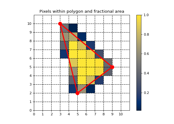
Single Polygons

The px and py arguments are used to pass in the x and y coordinates of the polygon vertices. For example,

import matplotlib.pyplot as plt
import numpy as np
from sofia_redux.toolkit.image.fill import polyfillaa

# Define a polygon
px = [5, 3, 9]
py = [2, 10, 5]

pixels, areas = polyfillaa(px, py, area=True)
grid = np.full((11, 11), np.nan)
grid[pixels[:, 0], pixels[:, 1]] = areas

fig, ax = plt.subplots(figsize=(7, 5))
ax.set_xticks(np.arange(-0.5, 10, 1))
ax.set_yticks(np.arange(-0.5, 10, 1))
ax.set_xticklabels(np.arange(11))
ax.set_yticklabels(np.arange(11))

ax.grid(which='major', axis='both', linestyle='--',
        color='k', linewidth=1)
img = ax.imshow(grid, cmap='cividis', origin='lower')

ax.plot(np.array(px + [px[0]]) - 0.5, np.array(py + [py[0]]) - 0.5,
        '-o', color='red', linewidth=3, markersize=10)
fig.colorbar(img, ax=ax)
ax.set_title("Pixels within polygon and fractional area")

(Source code, png, hires.png, pdf)

In the above plot, the fraction of pixel within the triangle is color coded.

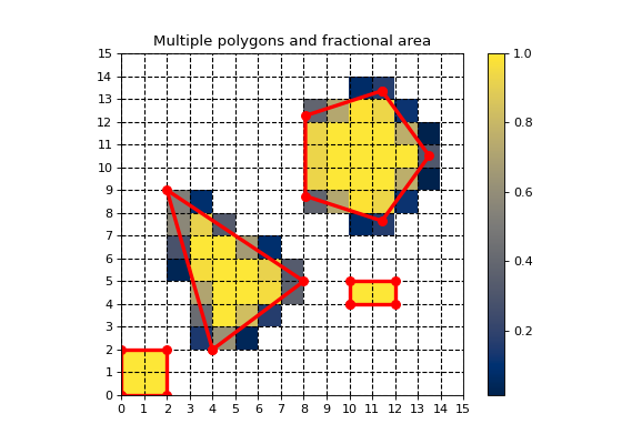
Multiple Polygons

If multiple polygons are to be calculated, there are two ways of indicating which points belong to which polygons. The first method allows px and py to still be provided as 1-dimensional arrays, but an additional parameter start_indices, is used to provide the starting index of each polygon within. For example:

px = [0, 0, 2, 2, 4, 2, 8, 12, 12, 14, 14]
py = [0, 2, 2, 0, 2, 9, 5,  4,  5,  5,  4]
#    |-- 0 ----||--- 1 --||------2-------|
start_indices = [0, 4, 7]

The second method uses a 2-level nested list, where each sublist contains the points for a polygon. For example:

px = [[0, 0, 2, 2], [4, 2, 8], [12, 12, 14, 14]]
py = [[0, 2, 2, 0], [2, 9, 5], [4,  5,  5,  4]]

The above examples all define the same shapes. The first is a square with vertices at (0, 0) (0, 2) (2, 2) (2 0), the second is a triangle (5, 2) (3, 9) (9, 5), and the list is a rectangle (100, 300) (100, 400) (200, 400) (200, 300).

Results will be output as a dict as discribed above. For example:

from sofia_redux.toolkit.image.fill import polyfillaa
import numpy as np
import matplotlib.pyplot as plt

px = [[0, 0, 2, 2], [4, 2, 8], [10, 10, 12, 12]]
py = [[0, 2, 2, 0], [2, 9, 5], [4,  5,  5,  4]]

# Add a pentagon
def mypoly(x, y, r, n):
    ang = (np.arange(n) + 1) * 2 * np.pi / n
    return list(r * np.cos(ang) + x), list(r * np.sin(ang) + y)

hx, hy = mypoly(10.5, 10.5, 3, 5)
px.append(hx)
py.append(hy)

result, areas = polyfillaa(px, py, area=True)

grid = np.full((15, 15), np.nan)
for i in range(len(result.keys())):
    grid[result[i][:,0], result[i][:,1]] = areas[i]

fig, ax = plt.subplots(figsize=(7, 5))
ax.set_xticks(np.arange(-0.5, 15, 1))
ax.set_yticks(np.arange(-0.5, 15, 1))
ax.set_xticklabels(np.arange(16))
ax.set_yticklabels(np.arange(16))

ax.grid(which='major', axis='both', linestyle='--',
        color='k', linewidth=1)
img = ax.imshow(grid, cmap='cividis', origin='lower')

for i in range(len(px)):
    x = px[i] + [px[i][0]]
    y = py[i] + [py[i][0]]
    ax.plot(np.array(x) - 0.5, np.array(y) - 0.5,
            '-o', color='red', linewidth=3, markersize=7)

fig.colorbar(img, ax=ax)
ax.set_title("Multiple polygons and fractional area")

(Source code, png, hires.png, pdf)

Note, that the center of a pixel cell is defined at (x + 0.5, y + 0.5) while (x, y) is defined as the bottom-left corner of a pixel cell. matplotlib defined (x, y) as the center of a cell, which is why there are various 0.5 corrections dotted throughout the examples above for plotting.