Image Warping through polynomial transformation

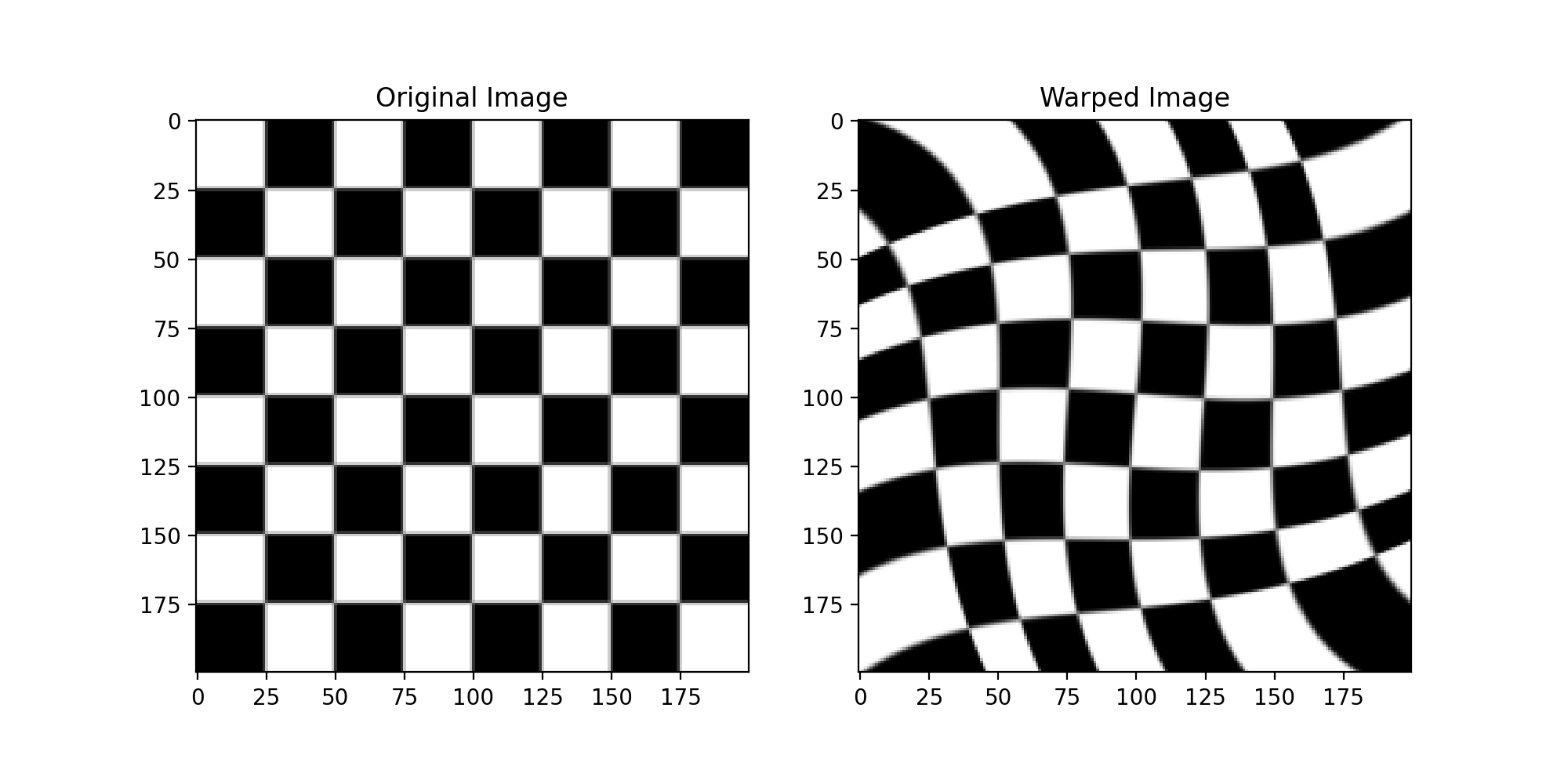
Image warping can be achieved using the warp_image() function. Here, two sets of coordinates should be provided: one indicating a standard set of (x, y) coordinates; the other giving those same coordinates at a warped location. Note that NaN handling is available for warp_image(). The following warps an image in which pixels are rotated according from their distance from the center:

import numpy as np
import matplotlib.pyplot as plt
import imageio
from sofia_redux.toolkit.image.warp import warp_image

image = imageio.imread('imageio:checkerboard.png')
sy, sx = image.shape

# Define some original grid positions
xi, yi = np.meshgrid(np.linspace(0, sx, sx // 20),
                     np.linspace(0, sy, sy // 20))

# Define some rotated grid positions
cenx, ceny = sx / 2, sy / 2
xo = xi - cenx
yo = yi - ceny
r = np.sqrt((xo ** 2) * (yo ** 2))
r /= r.max()
a = np.radians(-20) * r
xo = xo * np.cos(a) - yo * np.sin(a)
yo = xo * np.sin(a) + yo * np.cos(a)
xo += cenx
yo += ceny

# create a new image on the rotated coordinates
rotated = warp_image(image, xi, yi, xo, yo, mode='edge')

plt.figure(figsize=(10, 5))
plt.subplot(121)
plt.imshow(image, cmap='gray')
plt.title("Original Image")

plt.subplot(122)
plt.imshow(rotated, cmap='gray')
plt.title("Warped Image")

(Source code, png, hires.png, pdf)

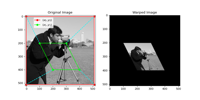
Polynomial Image Warping

The polywarp() function is functionally equivalent to the IDL polywarp function. It returns the \(K_x\) and \(K_y\) coefficients that describe the transformation of coordinates \((x_0, y_0)\) onto \((x_1, y_1)\) such that

\begin{eqnarray} x_1 & = & \sum_{i, j} K_{x_{i, j}} x_0^j y_0^i \\ y_1 & = & \sum_{i, j} K_{y_{i, j}} x_0^j y_0^i \end{eqnarray}

For example:

>>> from sofia_redux.toolkit.image.warp import polywarp
>>> x0 = [61, 62, 143, 133]
>>> y0 = [89, 34, 38, 105]
>>> x1 = [24, 35, 102, 92]
>>> y1 = [81, 24, 25, 92]
>>> kx, ky = polywarp(x1, y1, x0, y0, order=1)
>>> kx, ky
(array([[-5.37841592e+00, -3.20945283e-01],
        [ 7.51471270e-01,  2.22928691e-03]]),
 array([[-1.01479518e+01,  1.07084966e+00],
        [-1.68754432e-02, -5.76213991e-04]]))

Since this formulation of polynomial coefficients does not fit into the standard sofia_redux.toolkit.polynomial API, a special use case function, polywarp_image() can be used to call and apply the results of polywarp().

Firstly, polynomial coefficients are derived using polywarp() followed by interpolation (through sofia_redux.toolkit.interpolate.Interpolate) of the original image onto a newly defined warped set of coordinates. For example:

from sofia_redux.toolkit.image.warp import polywarp_image
import matplotlib.pyplot as plt
import imageio

image = imageio.imread('imageio:camera.png')
# Define warp based on corners of image for this example
x0 = [0, 0, 511, 511]
y0 = [511, 0, 0, 511]
x1 = [200, 100, 300, 400]
y1 = [400, 200, 200, 400]
warped = polywarp_image(image, x0, y0, x1, y1)

fig, ax = plt.subplots(nrows=1, ncols=2, figsize=(10, 5))
ax[0].imshow(image, cmap='gray')
ax[0].set_title("Original Image")
ax[0].set_xlim(-10, 521)
ax[0].set_ylim(521, -10)
ax[0].plot(x0 + [x0[0]], y0 + [y0[0]], '-o', color='red', markersize=6,
           label="$(x_0, y_0)$")
ax[0].plot(x1 + [x1[0]], y1 + [y1[0]], '-o', color='lime', markersize=6,
           label="$(x_1, y_1)$")
for i in range(4):
    ax[0].plot([x0[i], x1[i]], [y0[i], y1[i]], '--', color='cyan')

ax[0].legend(loc=(0.12, 0.82))
ax[1].imshow(warped, cmap='gray')
ax[1].set_title("Warped Image")

(Source code, png, hires.png, pdf)

If warping is required in more than two dimensions, similar results could be achieved using a combination of sofia_redux.toolkit.fitting.polynomial.Polyfit and sofia_redux.toolkit.interpolate.Interpolate.