Generally, polynomial algorithms in the sofia_redux.toolkit.fitting module either fit polynomial coefficients to a sample distribution, or evaluate polynomial coefficients at a given location. The polyfitnd() function is used to derive polynomial coefficients, while poly1d() or polynd() functions evaluate coefficients in 1 or N dimensions respectively. The Polyfit class is capable of both deriving and evaluating polynomials. However, if one only wishes to derive and then evaluate a polynomial fit to data (i.e. resample) but does not require the actual coefficients using piecewise fits, it is recommended to instead refer to sofia_redux.toolkit.resampling, developed for just that purpose.

Polynomial Coefficients

In this scheme, coefficients are stored as an N-dimensional array with the size of each dimension equal to the polynomial degree (order + 1) set for that dimension. For example, if we wish to fit a set of 2-dimensional data with a 2nd order (degree=3) polynomial in x, and a 3rd order (degree=4) polynomial in y, an array of shape (3, 4) would be used to contain the polynomial coefficients necessary to model the data with the desired polynomial.

Polynomial functions model distribution \(x\) as:

\[f(x) = \sum_{p_{1}=0}^{o_{1}} \sum_{p_{2}=0}^{o_{2}} ... \sum_{p_{N}=0}^{o_{N}} a_{(p_{1},p_{2},...,p_{N})} x_{1}^{p_{1}} x_{2}^{p_{2}} ... x_{N}^{p_{N}}\]

in \(N\) dimensions where \(o_{i}\) is the polynomial order fitted to dimension \(i\), and \(a\) are the polynomial coefficients. For example, polynomial coefficients could be used to model the function

\[f(x) = 5 + 2x + 3xy + 0.5y^{2}\]

as

\[\begin{split}a = \begin{bmatrix} 5 & 2 & 0 \\ 0 & 3 & 0 \\ 0.5 & 0 & 0 \end{bmatrix}\end{split}\]

using a second order polynomial in both x and y.

The following example uses polyfitnd() to derive these coefficients:

from sofia_redux.toolkit.fitting.polynomial import polyfitnd
import numpy as np

y, x = np.mgrid[:5, :5]
z = 5 + (2 * x) + (3 * x * y) + (0.5 * y ** 2)
a = polyfitnd(x, y, z, 2)
assert np.allclose(a, [[5, 2, 0],
                       [0, 3, 0],
                       [0.5, 0, 0]])

These coefficients can then be evaluated using polynd():

from sofia_redux.toolkit.fitting.polynomial import polynd

fitted = polynd(np.stack((y, x)), a)
assert np.allclose(z, fitted)

Both derivation and evaluation can be performed by the Polyfit class:

from sofia_redux.toolkit.fitting.polynomial import Polyfit

pfit = Polyfit(x, y, z, 2)
assert np.allclose(pfit.get_coefficients(), a)
assert np.allclose(pfit(x, y), z)

Please note however, that in all the above examples, we have used the default redundant polynomial representation such that no coefficients will be calculated for \(a\) when \(\sum_{i=1}^{N}{p_i} > max(o)\). So for a redundant (default) polynomial fit of order 2 in both dimensions

\[\begin{split}a = \begin{bmatrix} 5 & 2 & 0 \\ 0 & 3 & - \\ 0.5 & - & - \end{bmatrix}\end{split}\]

where values marked with \(-\) will always be set to zero since they are defined as redundant.

This default redundancy behaviour may be overridden by explicitly providing terms for which coefficients must be derived. The format of these terms should be provided as an integer array of shape (n_terms, n_dimensions), with each value corresponding to the power of a single term in a specific dimension. For example, in 3-dimensions, the value [1, 2, 3] would result in a coefficient being calculated for term \(xy^2z^3\). The sofia_redux.toolkit.utilities.func.polyexp() may be used for the purposes of creating either full or redundant set of terms.

from sofia_redux.toolkit.fitting.polynomial import polyexp
# Create a redundant set of terms
redundant = polyexp(2, ndim=2)
print(redundant)
# [[0 0]
#  [1 0]
#  [2 0]
#  [0 1]
#  [1 1]
#  [0 2]]

The above redundant set results in a function of the form:

\[f(x) = a_{0,0} + a_{1,0}x + a_{2,0}x^2 + a_{0,1}y + a_{1,1}xy + a_{0,2}y^2\]

# Create a full set of terms
full = polyexp([2, 2])
print(full)
# [[0 0]
#  [1 0]
#  [2 0]
#  [0 1]
#  [1 1]
#  [2 1]
#  [0 2]
#  [1 2]
#  [2 2]]

The above full set results in a function of the form:

\[f(x) = a_{0,0} + a_{1,0}x + a_{2,0}x^2 + a_{0,1}y + a_{1,1}xy + a_{2,1}x^2y + a_{0,2}y^2 + a_{1,2}xy^2 + a_{2,2}x^2y^2\]

Alternatively, terms may be explicitly defined by the user:

user = [[2, 0], [1, 1]]

In this case, the user has specified that coefficients should only by derived for the terms in the following function:

\[f(x) = a_{2,0}x^2 + a_{1,1}xy\]

For example, attempting to fit the function

\[f(x) = 1 + 2xy + 0.1x^2y^2\]

can only be done with either a full or user defined set of terms since \(x^2y^2\) will never appear in a redundant set of a 2nd order 2-dimensional polynomial function:

y, x = np.mgrid[:5, :5]
z = 1 + (2 * x * y) + (0.1 * x ** 2 * y ** 2)

redundant_pfit = Polyfit(x, y, z, 2)
print(redundant_pfit.get_coefficients().round(decimals=2))
# [[ 3.8 -3.2  0.6]
#  [-3.2  3.6  0. ]
#  [ 0.6  0.   0. ]]

full_pfit = Polyfit(x, y, z, polyexp([2, 2]), set_exponents=True)
print(full_pfit.get_coefficients().round(decimals=2))
# [[ 1.  -0.   0. ]
#  [-0.   2.  -0. ]
#  [ 0.  -0.   0.1]]

user_pfit = Polyfit(x, y, z, [[0, 0], [1, 1], [2, 2]], set_exponents=True)
print(user_pfit.get_coefficients().round(decimals=2))
# [[1.  0.  0. ]
#  [0.  2.  0. ]
#  [0.  0.  0.1]]

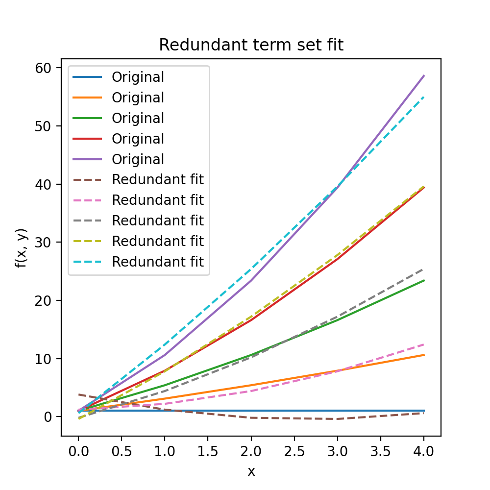
As can be seen above, the default redundant set of terms failed to derive the correct coefficients, but made its best attempt using those terms available. The full and user defined sets both returned the correct values. Note that in order to override the default redundant behaviour, set_exponents=True must be set as a keyword argument. Also note that while the redundant fit failed, the resulting fit is the “best fit” with the terms available as can be seen below:

import matplotlib.pyplot as plt
import numpy as np
from sofia_redux.toolkit.fitting.polynomial import Polyfit

y, x = np.mgrid[:5, :5]
z = 1 + (2 * x * y) + (0.1 * x ** 2 * y ** 2)
redundant_pfit = Polyfit(x, y, z, 2)

plt.figure(figsize=(5, 5))
plt.plot(z, label='Original')
plt.plot(redundant_pfit(x, y), '--', label="Redundant fit")
plt.xlabel('x')
plt.ylabel('f(x, y)')
plt.title("Redundant term set fit")
plt.legend()

(Source code, png, hires.png, pdf)

Plots for the full and user defined sets would reproduce the original data.

Fit Statistics

In addition to performing and evaluating a polynomial fit, Polyfit can also return useful statistics including covariance terms. The Polyfit.stats attribute is a namespace containing the following statistics:

• n: Number of samples

• dof: Degrees of Freedom

• fit: An array containing the fit to the original data

• residuals: An array containing the difference between the data and the fit

• sigma: An array containing the error of each polynomial coefficient

• rms: The root-mean-square error on the fit

• chi2: The \(\chi^2\) statistic on the fit

• rchi2: The reduced \(\chi^2\) statistic on the fit

• q: Goodness of fit, or survival function. The probability (0->1) that

  one of the samples is greater than \(\chi^2\) away from the fit.

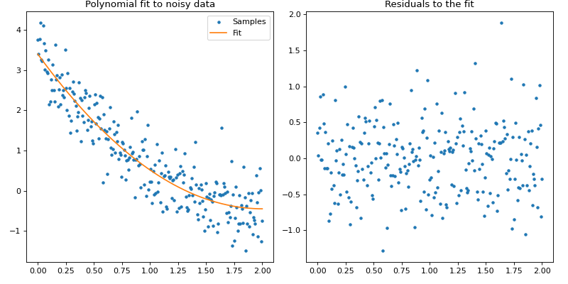
These can be accessed directly or printed to screen by applying the standard Python print() function to an initialized Polyfit object. For example:

import numpy as np
import matplotlib.pyplot as plt
from sofia_redux.toolkit.fitting.polynomial import Polyfit

# Create function
x = np.linspace(0, 2, 256)
y = -0.5 + (x - 2) ** 2

# add noise with a normal distribution
rand = np.random.RandomState(42)
noise = rand.normal(loc=0, scale=0.5, size=x.size)
y += noise

# Fit a 2nd order polynomial to the noisy data
# Since we know the scale of the error, it may be included
pfit = Polyfit(x, y, 2, error=0.5)

fig, ax = plt.subplots(nrows=1, ncols=2, figsize=(10, 5))
fig.tight_layout()
ax[0].plot(x, y, '.', label="Samples")
ax[0].plot(x, pfit.stats.fit, '-', label="Fit")
ax[0].legend()
ax[0].set_title("Polynomial fit to noisy data")
ax[1].plot(x, pfit.stats.residuals, '.')
ax[1].set_title("Residuals to the fit")

print(pfit)

(Source code, png, hires.png, pdf)

Textual output:

Name: Polyfit

         Statistics
--------------------------------
Number of original points : 256
           Number of NaNs : 0
       Number of outliers : 0
     Number of points fit : 256
       Degrees of freedom : 253
              Chi-Squared : 240.743406
      Reduced Chi-Squared : 0.951555
      Goodness-of-fit (Q) : 0.300082
     RMS deviation of fit : 0.485822

    Exponents : Coefficients
--------------------------------
(0,) : 3.396036 +/- 0.093022
(1,) : -3.840006 +/- 0.214879
(2,) : 0.958356 +/- 0.104002

Covariance

The full covariance matrix is available in the Polyfit.covariance attribute. Note that this is an (n_coefficient, n_coefficient) giving the covariance between terms, with each axis ordered in the same manner as the terms. The order of the terms can be determined from the Polyfit.exponents attribute. For example:

import numpy as np
from sofia_redux.toolkit.fitting.polynomial import Polyfit

# Create a function
y, x = np.mgrid[:10, :10]
z = 1 - (5 * x) + (3 * y)
pfit = Polyfit(x, y, z, 1)
print("Exponents:\n%s\n" % pfit.exponents)
print("Covariance:\n%s" % pfit.covariance)

Output:

Exponents:
[[0 0]
 [1 0]
 [0 1]]

Covariance:
[[ 5.90909091e-02 -5.45454545e-03 -5.45454545e-03]
 [-5.45454545e-03  1.21212121e-03  4.33680869e-19]
 [-5.45454545e-03 -0.00000000e+00  1.21212121e-03]]

In the above example, the rows and columns of the covariance matrix are ordered as \(a_{0,0}, a_{1, 0}, a_{0,1}\) for the terms \(x^0y^0, x, y\).

Disabling Statistics

If statistics are not required, there is no need for a covariance matrix, and processing speed is important, statistical calculations may be disabled by setting stats=False and/or covar=False during intialization. If statistics are disabled, they will no longer be calculated or displayed. If covariance calculations are disabled, the Polyfit.covariance attribute will be set to None.

import numpy as np
from sofia_redux.toolkit.fitting.polynomial import Polyfit

y, x = np.mgrid[:10, :10]
z = 1 - (5 * x) + (3 * y)
pfit = Polyfit(x, y, z, 1, stats=False, covar=False)
assert pfit.covariance is None
print(pfit)

Output:

Name: Polyfit

    Exponents : Coefficients
--------------------------------
(0, 0) : 1.000000
(1, 0) : -5.000000
(0, 1) : 3.000000

However, if robust outlier rejection is enabled, by necessity, both statistics and covariance will be calculated regardless of user wishes.

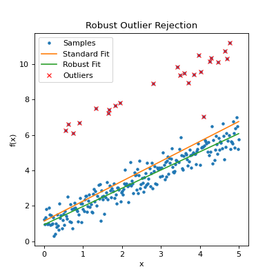
Robust Outlier Rejection

Robust outlier rejection may be enabled by setting robust > 0 during Polyfit initialization. If set, outliers are identified through an iterative process: fitting the data then excluding any samples that fall outside robust sigmas from the fit before repeating. Iterations are terminated after:

1. A certain number of iterations have occurred.

2. The relative delta between successive residual RMS values is less than a set value.

4. Too many samples are excluded such that fitting the desired order of polynomial will not be possible.

5. The fit failed.

Whether the iteration succeeded can be determined from the Polyfit.success attribute, while the termination condition encountered is in the Polyfit.termination attribute. Which samples were excluded during the rejection process can be determined from the Polyfit.mask attribute. Additional statistics will also be displayed if statistics are printed to screen. For example:

import numpy as np
from sofia_redux.toolkit.fitting.polynomial import Polyfit

# Create a function
x = np.linspace(0, 5, 256)
y = 1 + x
rand = np.random.RandomState(42)

# Add noise
noise = rand.normal(loc=0, scale=0.5, size=y.shape)
y += noise

# Add some obvious outliers, throwing off the fit
inds = rand.randint(0, 255, 25)
y[inds] += 5

# Standard fit
pfit = Polyfit(x, y, 1)

# Robust fit with 3 sigma outlier rejection
rfit = Polyfit(x, y, 1, robust=3)
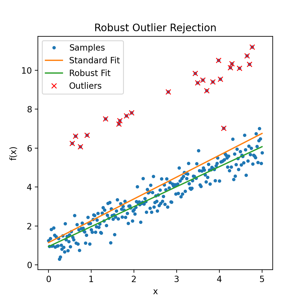
outliers = np.argwhere(~rfit.mask)[:, 0]

plt.figure(figsize=(5, 5))
plt.plot(x, y, '.', label='Samples')
plt.plot(x, pfit.stats.fit, label='Standard Fit')
plt.plot(x, rfit.stats.fit, label='Robust Fit')
plt.plot(x[outliers], y[outliers], 'x', color='red', label='Outliers')
plt.title("Robust Outlier Rejection")
plt.xlabel("x")
plt.ylabel("f(x)")
plt.legend()

# Display robust statistics
print(rfit)

(Source code, png, hires.png, pdf)

Output:

Name: Polyfit

         Statistics
--------------------------------
Number of origial points : 256
          Number of NaNs : 0
      Number of outliers : 24
    Number of points fit : 232
      Degrees of freedom : 230
             Chi-Squared : 53.825532
     Reduced Chi-Squared : 0.234024
     Goodness-of-fit (Q) : 0.000000
    RMS deviation of fit : 0.482712
 Outlier sigma threshold : 3
 eps (delta_sigma/sigma) : 0.01
              Iterations : 3
   Iteration termination : delta_rms = 0

    Exponents : Coefficients
--------------------------------
(0,) : 0.941421 +/- 0.129497
(1,) : 1.026215 +/- 0.045540

The above report indicates 24 outliers were found in which the residual was greater than the \(3\sigma\) limit. 3 iterations were required, terminated when no further outliers could be found (delta_rms = 0).

Special Case 1-D and 2-D Functions

For quick and easy derivation and evaluation of polynomial coefficients in one or two dimensions, several functions are available that deviate from the more general API presented above.

1-Dimensional Polynomial Derivation and Evaluation

For fitting a 1-dimensional polynomial to data where no special considerations are necessary, there are already many functions available in standard Python packages such as numpy.polyfit(), so no attempt has been made to recreate another version. polyfit() is perfectly capable of handling 1 dimensional cases with the added benefits of sofia_redux.toolkit.fitting.polynomial.Polyfit functionality.

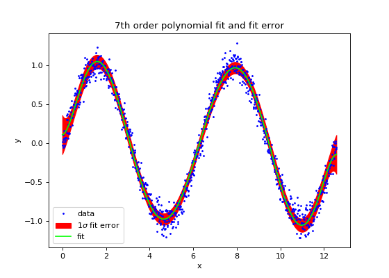
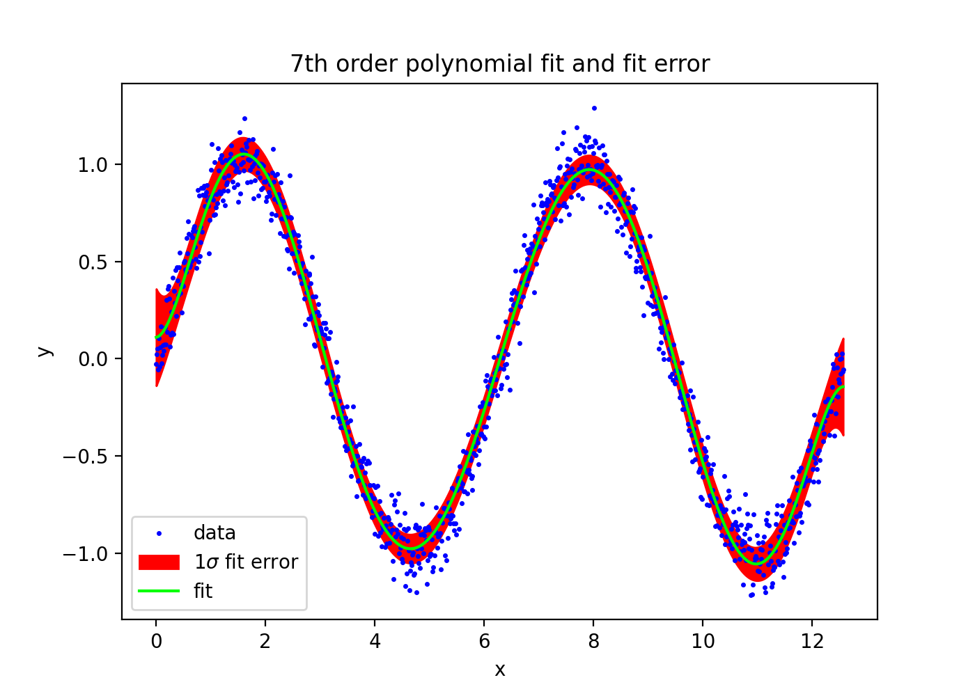
However, for 1-dimensional evaluation, poly1d() is available to evaluate coefficients, and optional variance if either the full covariance matrix is provided, or the diagonal of the covariance matrix is given.

import numpy as np
import matplotlib.pyplot as plt
from sofia_redux.toolkit.fitting.polynomial import poly1d, polyfitnd

x = np.linspace(0, 4 * np.pi, 1000)
y = np.sin(x)
error = np.random.RandomState(41).normal(loc=0, scale=0.1, size=x.size)
y += error

# use polyfitnd to fit a polynomial and get the covariance on the fit
# coefficients
coeffs, cvar = polyfitnd(x, y, 7, covar=True)
yfit, yvar = poly1d(x, coeffs, covar=cvar)
error = np.sqrt(yvar)

plt.figure(figsize=(7, 5))
plt.plot(x, y, '.', markersize=3, label='data', color='blue')
plt.fill_between(x, yfit - error, yfit + error, color='red',
                 label=r'$1\sigma$ fit error')
plt.plot(x, yfit, label='fit', color='lime')
plt.legend(loc='lower left')
plt.title("7th order polynomial fit and fit error")
plt.xlabel('x')
plt.ylabel('y')

(Source code, png, hires.png, pdf)

Please note that polynd() and Polyfit are both capable of producing the same results as poly1d(). However, poly1d() is a lighter version using numpy.poly1d() to evaluate coefficients rather than the engine used by polynd().

2-Dimensional Polynomial Derivation and Evaluation

For 2-dimensional data, the polyfit2d() and poly2d() distinguish between the full set of polynomial coefficients, and the more robust redundancy controlled term coefficients in the same way as polyfitnd(). This distinction is controlled by the full keyword. The following table gives an example of the coefficients for a 2^nd order polynomial with full=True and full=False. Note that the order of coefficients in the output table is different from polyfitnd(), with x coefficients running along columns and y coefficients by rows, where the exponent of the coefficient term is given by it’s index. The order of polynomial must be given separately for the x and y directions via the kx and ky keyword arguments (default=2).

Table 2 Polynomial Coefficients (full=True)

	x0	x1	x2
y0	c0,0	c1,0	c2,0
y1	c0,1	c1,1	c2,1
y2	c0,2	c1,2	c2,2

Table 3 Polynomial Coefficients (full=False)

	x0	x1	x2
y0	c0,0	c1,0	c2,0
y1	c0,1	c1,1
y2	c0,2

2-Dimensional Examples

• polyfit2d() derives polynomial coefficients describing a surface:

  >>> import numpy as np
  >>> from sofia_redux.toolkit.fitting.polynomial import polyfit2d
  >>> y, x = np.mgrid[:5, :5]
  >>> z = 0.5 + (0.4 * x) + (0.3 * y) + (0.2 * x * y) + (0.1 * x ** 2)
  >>> c = polyfit2d(x, y, z, kx=2, ky=2)
  >>> print(np.abs(np.round(c, decimals=3)))
  [[0.5 0.4 0.1]
   [0.3 0.2 0. ]
   [0.  0.  0. ]]
  

• poly2d() evaluates 2-dimensional polynomial coefficients:

  >>> from sofia_redux.toolkit.fitting.polynomial import poly2d
  >>> np.allclose(poly2d(x, y, c), z)
  True
  

• polyinterp2d() derivates and evaluates 2-D polynomial coefficients:

  >>> from sofia_redux.toolkit.fitting.polynomial import polyinterp2d
  >>> np.allclose(polyinterp2d(x, y, z, x, y, ky=2, kx=2), z)
  True
  

These 2-dimensional functions are designed as lighter versions of polyfitnd() and polynd(), so should fit and evaluate data slightly faster.