fitpeaks1d() is designed to fit a signal, or superimposed signals, along with a background to 1-dimensional data. It is essentially a wrapper for the astropy.modeling module allowing for customization, and ease of use for the most common case uses (developed using astronomical data). The algorithm is divided into three phases: the search phase, an initial baseline estimate, and the refined fitting phase:

Search Phase

The purpose of the search phase is to get a good approximation of peak locations in the data along the independent axis. These may be supplied by the user (e.g. known apertures), or an estimate may be made. Estimates are made using the following process:

1. Processing function (Optional)

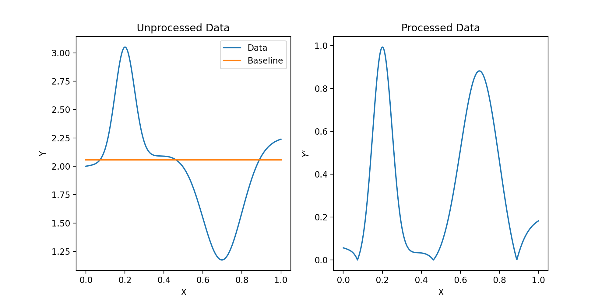
Apply a processing function to \((x, y)\) data to return a approximate baseline and new dependent values (\(y^{\prime}\)) for the subsequent step to operate on. The default processing function (medabs_baseline()) subtracts the median y value and then returns absolute values:

\[y^{\prime} = | y - median(y) |\]

(Source code, png, hires.png, pdf)

The default medabs_baseline() function is just designed to be a general usage quick function to handle positive and negative peaked signals. This may be not be suitable for some data sets in which case the user should write their own function that takes in (x, y) and returns (\(y^{\prime}\), baseline) where all inputs and outputs are 1-D numpy arrays of the same size.

2. Guess function (Optional)

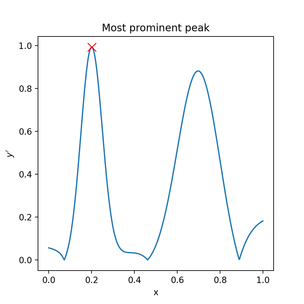
The next step passes \((x, y^{\prime}\) to the guess function which should be designed to return a quick estimate of the x and y value for the most prominent peak \((x_{peak}, y^{\prime}_{peak}) `in :math:`y^{\prime}\) (not \(y\)). The default guess function (guess_xy_mad()) is designed to work with the default processing function (medabs_baseline()). Therefore, if changing one, be considerate of the other. medabs_baseline() returns the following:

\begin{eqnarray} y_{peak} & = & max(|y^{\prime} - median(y^{\prime}) | ) \\ x_{peak} & = & x \, | \, y^{\prime}(x) = y_{peak} \end{eqnarray}

(Source code, png, hires.png, pdf)

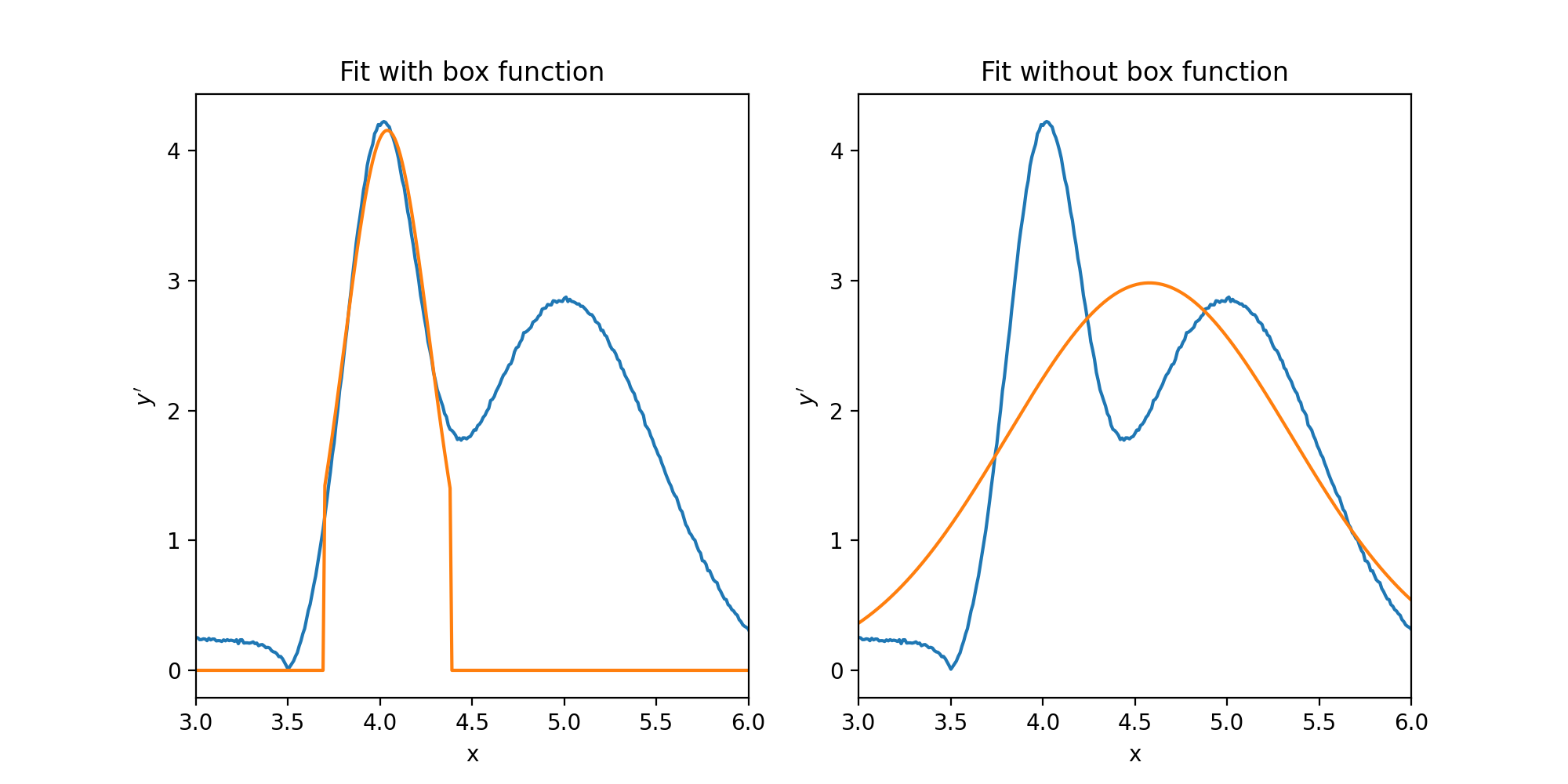
3. Rough Initial Parameter Estimation and the Box Function

A fit is then performed at either the most prominent peak identified in steps 1 and 2, or the first user supplied guess position. The parameters determined here will be used as initialization parameters for the final fitting and also (if required), to search for other peaks in the data. When fitting peaks that are close together, or the data has structure in the baseline, it can be important to use a box function to limit the range of the fitting along \(x\). Initial fits to the most prominent peak are shown below with and without the boxing function.

(Source code, png, hires.png, pdf)

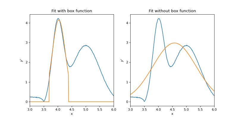
There are a couple of things to note above. Firstly, the fit on the right (without a box function) has fit both peaks present in the data with a single Gaussian, which is obviously incorrect. Secondly, the fit on the left did not fit the peak very well, which is why a second more refined fit occurs at a later stage. Clipping of the fit due to the box function can also be seen in the left plot. Finally, while the initial fit on the right failed, there is still a good chance that the final fit will still fit the data correctly since this is a fairly simple model.

The default box function is a astropy.modeling.models.Box1D with a width of 6 times the width parameter of the peak function (fwhm in the case of the default astropy.modeling.models.Gaussian1D). However, since it will not always be the case that we wish to fit Gaussians, or that the best way to separate one peak from another is a standard box (hat) function, the box function, the peak width parameter and it’s relationship to the width of the box function can be configured. The box model must be a astropy.modeling.Fittable1DModel and is passed into fitpeaks1d() with the box_class parameter.

The box_width parameter can either be a single float or int value, in which case the width if the box will be held fixed (in units of \(x\)). Alternatively, a tuple of the form (peak_parameter_name, width) can be supplied indicating that the width of the box should always a width multiple of certain parameter of the peak model. More complex relationships can also be defined through the search_kwargs parameter which will be described later.

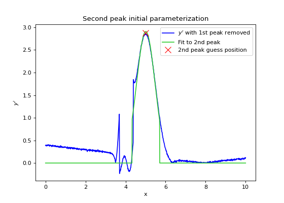
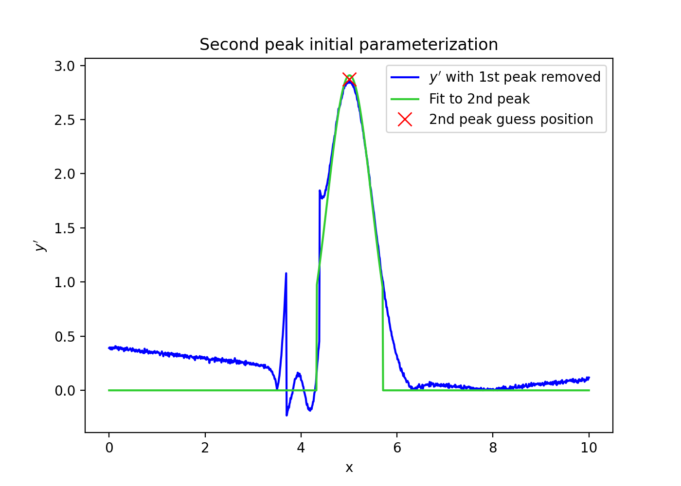
4. Identify remaining peaks

Once the first or most prominent peak has undergone initial parameterization, it’s fit will be subtracted from \(y^{\prime}\) and steps 1-3 will be repeated do identify up to npeaks (default=1) peaks. If more than one peaks are to be identified, this MUST be specified by the user. If automatically detecting peaks, peaks will be fit in the order of most prominent to least as determined from the initial search phase. Otherwise, if guess positions were supplied by the user, peaks will be fit in the supplied order.

(Source code, png, hires.png, pdf)

Initial Baseline Fitting

Once estimates of the peak parameters have been determined from the search phase, they are used to initialize a final model comprising of npeaks peaks and an optional baseline. By default, a constant offset value will be used to model the baseline (astropy.modeling.models.Const1D) although any astropy.modeling.Fittable1DModel may be used if passed into via the background_class keyword argument.

Before final fitting, the user may process the data one final time in a similar way to baseline_func using the optional_func keyword argument to pass in a function of the form \(y^{\prime} = f(x, y)\). There are not many instances when one may want to do this, except for possibly filtering or smoothing the initial data.

Next, if the user has requested a baseline fit, a fit may be performed to initialize the background component of the final model. This baseline fit will be performed on the residual between the initial peak fit and the original data. Alternatively, the user may supply expected background parameters. For example, offset for a constant background or slope and offset for a linear function. These may be supplied through the binit keyword argument.

(Source code, png, hires.png, pdf)

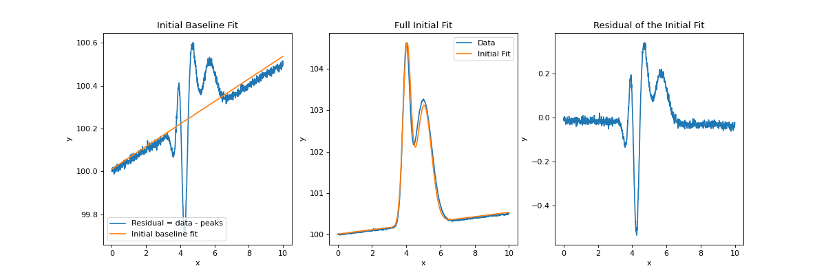
The above plot shows an initial baseline fit on the residual of the data to the initial peak fits on the left, and the initialized model generated from the peak and baseline approximation on the right. As can be seen, the model does show some discrepancy from the actual data, but provides a good starting point for a final fit to be performed.

Final Refined Fit

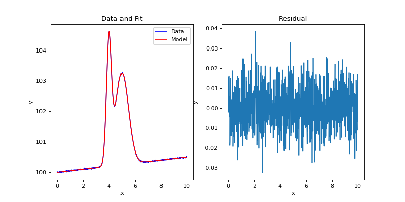
Finally, a new model, initialized by the previous peak and baseline fits is used as a starting point to fit the full model and baseline in it’s entirety. This time, no boxing function is applied as we will have hopefully untangled any compound peaks or confusing baseline structure in the previous steps. The code below runs all steps using the fitpeaks1d() function.

import numpy as np
import matplotlib.pyplot as plt
from astropy.modeling import models, fitting
from sofia_redux.toolkit.fitting.fitpeaks1d import fitpeaks1d

# Create some fake data with noise
x = np.linspace(0, 10, 1001)
model1 = models.Gaussian1D(amplitude=3, mean=5, stddev=0.5)
model2 = models.Gaussian1D(amplitude=4, mean=4, stddev=0.2)
y = model1(x) + model2(x) + 0.05 * x + 100
rand = np.random.RandomState(42)
y += rand.normal(0, 0.01, y.size)

model = fitpeaks1d(x, y, npeaks=2, background_class=models.Linear1D,
                   box_width=('stddev', 3),
                   search_kwargs={'stddev_0': 0.1})

fit = model(x)
fig, ax = plt.subplots(nrows=1, ncols=2, figsize=(10, 5))
ax[0].plot(x, y, label='Data', color='blue')
ax[0].plot(x, model(x), label='Model', color='red')
ax[0].legend()
ax[0].set_xlabel('x')
ax[0].set_ylabel('y')
ax[0].set_title("Data and Fit")
ax[1].plot(x, y - fit)
ax[1].set_xlabel('x')
ax[1].set_ylabel('y')
ax[1].set_title("Residual")

(Source code, png, hires.png, pdf)

Note that in the above example, search_kwargs={'stddev_0': 0.1} is used to set an initial value for the fwhm of each peak to 0.1 as if not specified, the default value for the astropy model will be used instead. In this case, for a astropy.modeling.models.Gaussian1D, the default value is 1 which is much too large for our expected peaks. Therefore, during the iterative fitting process, as fwhm is decreased, a local minimum in the cost function will be encountered by fitting both peaks with a single Gaussian, causing the iteration to stop at a result similar to the plot showing a fit without a box function. Also note that when using a boxing function during the search phase, peak name parameters are distinguished from box name parameters by the ‘_0’ suffix (stddev_0 in this case). Likewise, box name parameters are suffixed by ‘_1’.

Model Functionality

Once a model has been fit to the data, there are a few features that should hopefully be useful to the user:

Fit Information

The print() function can be used to display what the components of the model are, how they are related, and give parameter values. For example, using print on the above model generates the following:

>> print(model)
Model: CompoundModel
Name: 2_peaks_with_background
Inputs: ('x',)
Outputs: ('y',)
Model set size: 1
Expression: [0] + [1] + [2]
Components:
    [0]: <Gaussian1D(amplitude=2.99771258, mean=5.0000777, stddev=0.49993379)>

    [1]: <Gaussian1D(amplitude=4.00083062, mean=4.00004859, stddev=0.20010122)>

    [2]: <Linear1D(slope=0.05014067, intercept=99.99969687)>
Parameters:
       amplitude_0          mean_0      ...       slope_2         intercept_2
    ------------------ ---------------- ... ------------------- ----------------
    2.9977125792665062 5.00007770385712 ... 0.05014066710980406 99.9996968671665

This tells us that there are 3 components to our final model consisting of 2 peaks and one background. If a baseline was fit to the data, it will always exist as the last component of the model. Each component may be accessed through standard python indexing., i.e.:

peak1 = model[0]
peak2 = model[1]
baseline = model[2]

Again, each component can also display information to the user through print():

>> print(peak1)
Model: Gaussian1D
Inputs: ('x',)
Outputs: ('y',)
Model set size: 1
Parameters:
        amplitude            mean             stddev
    ------------------ ---------------- ------------------
    2.9977125792665062 5.00007770385712 0.4999337879214602

Parameter values may be extracted programmatically using the parameters attribute of the full model or any component model. Names of the parameters are stored in the param_names attribute. Note that parameter names are suffixed with “_n” if accessed from the full model where n indicates the component index. For example, “mean_1” would contain the mean \(x\) location of the 2nd Gaussian peak in the above examples. Component parameter names have no such suffix. Parameters may also be accessed through model attributes:

print(model.param_names[:3])
print(model[0].param_names)
assert np.allclose(model.parameters[:3], model[0].parameters)
assert np.equal(model.amplitude_0, model[0].amplitude)

Output:

('amplitude_0', 'mean_0', 'stddev_0')
('amplitude', 'mean', 'stddev')

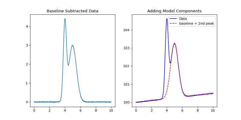
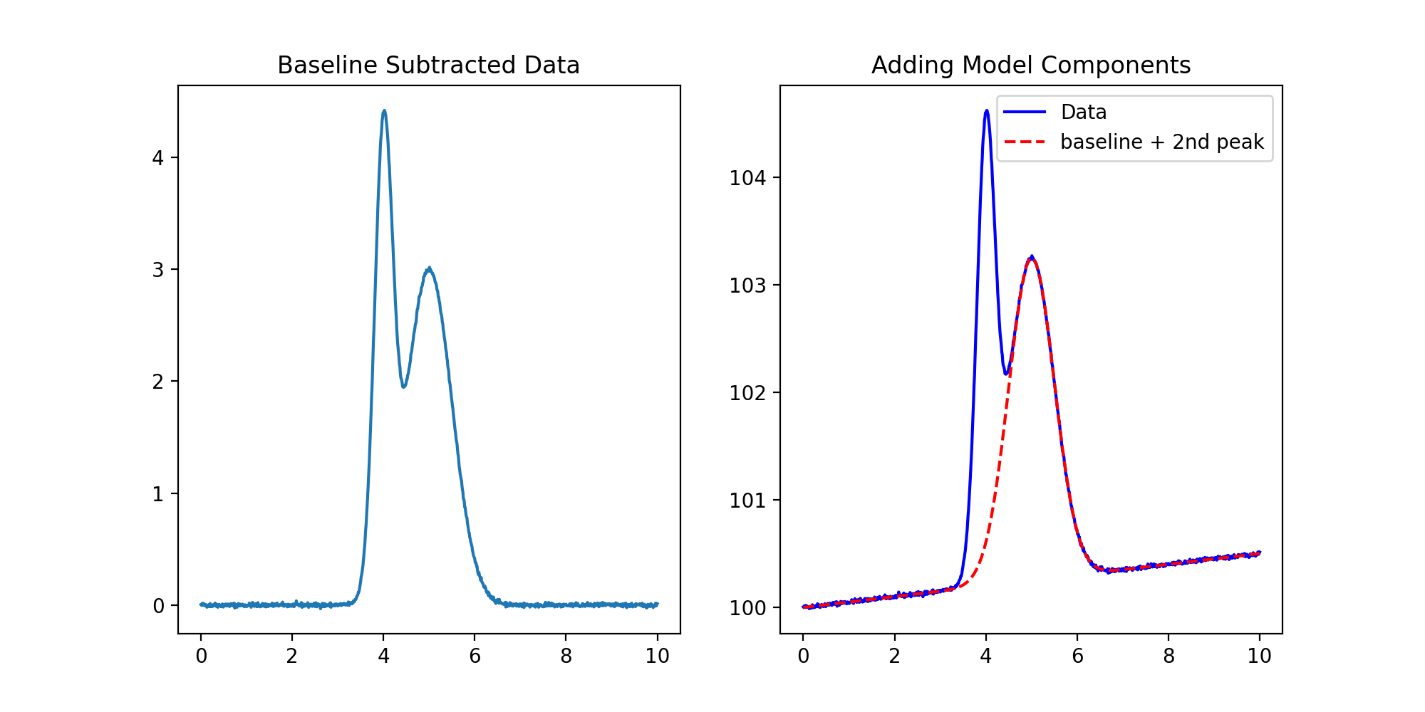
Evaluating Models

The full and component models may be evaluated at user supplied dependent variable locations. Standard arithmetic operations may also be performed on models (or components) to create new manipulations:

fig, ax = plt.subplots(nrows=1, ncols=2, figsize=(10, 5))
ax[0].plot(x, y - model[2](x))
ax[0].set_title('Baseline Subtracted Data')
ax[1].plot(x, y, label='Data', color='blue')
ax[1].plot(x, (model[0] + model[2])(x), '--',
           label='baseline + 2nd peak', color='red')
ax[1].set_title("Adding Model Components")
ax[1].legend()

(Source code, png, hires.png, pdf)

Further Examples

Large Baseline Structure (baseline_func usage and fixing known parameters)

import numpy as np
import matplotlib.pyplot as plt
from astropy.modeling import models
from sofia_redux.toolkit.fitting.fitpeaks1d import fitpeaks1d
from astropy.modeling.polynomial import Polynomial1D

x = np.linspace(0, 10, 1000)
baseline = 10 - (x - 5) ** 2
positive_source = models.Voigt1D(x_0=4, amplitude_L=5, fwhm_G=0.1)
negative_source = models.Voigt1D(x_0=7, amplitude_L=-5, fwhm_G=0.2)
rand = np.random.RandomState(41)
noise = rand.normal(loc=0, scale=1.5, size=x.size)
y = baseline + positive_source(x) + negative_source(x) + noise

def baseline_func(x, y):
    baseline = np.poly1d(np.polyfit(x, y, 2))(x)
    return np.abs(y - baseline), baseline

model = fitpeaks1d(x, y, npeaks=2,
                   peak_class=models.Voigt1D,
                   box_width=(None, 3),
                   background_class=Polynomial1D(2),
                   baseline_func=baseline_func)

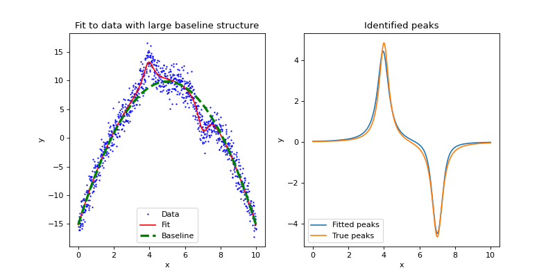
fig, ax = plt.subplots(nrows=1, ncols=2, figsize=(10, 5))
ax[0].plot(x, y, '.', label='Data', color='blue', markersize=2)
ax[0].plot(x, model(x), label='Fit', color='red')
ax[0].plot(x, model[2](x), '--', label='Baseline', color='green',
           linewidth=3)
ax[0].legend(loc='lower center')
ax[0].set_title("Fit to data with large baseline structure")
ax[0].set_xlabel('x')
ax[0].set_ylabel('y')
ax[1].plot(x, (model[0] + model[1])(x), label='Fitted peaks')
ax[1].plot(x, positive_source(x) + negative_source(x), label='True peaks')
ax[1].legend(loc='lower left')
ax[1].set_title("Identified peaks")
ax[1].set_xlabel('x')
ax[1].set_ylabel('y')
print(model)

(Source code, png, hires.png, pdf)

Output:

Model: CompoundModel
Name: 2_peaks_with_background
Inputs: ('x',)
Outputs: ('y',)
Model set size: 1
Expression: [0] + [1] + [2]
Components:
    [0]: <Voigt1D(x_0=7.00235917, amplitude_L=-10.44529587, fwhm_L=0.244132,
                  fwhm_G=0.57882632)>

    [1]: <Voigt1D(x_0=3.95826805, amplitude_L=5.05682365, fwhm_L=0.63766468,
                  fwhm_G=0.00500501)>

    [2]: <Polynomial1D(2, c0=-15.1200609, c1=10.00847117, c2=-1.00159934)>
Parameters:
          x_0_0          amplitude_L_0    ...        c1_2                c2_2
    ----------------- ------------------- ... ------------------ -------------------
    7.002359167002396 -10.445295870401356 ... 10.008471173888237 -1.0015993391982998

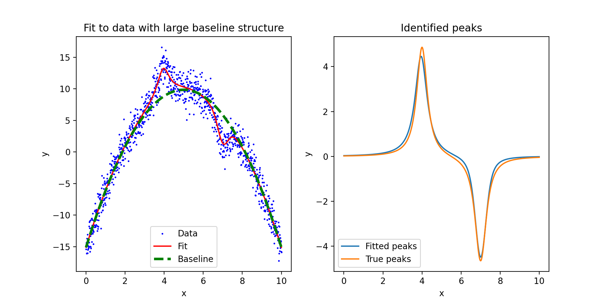
In the above example, a synthetic data set was generated where the structure of the baseline would confuse a naive fit. fitpeaks1d() is used to overcome this by defining baseline_func for use during the search phase. This user-defined function subtracts a 2nd order polynomial fit to the data as an estimate of the baseline, and also returns the absolute values of the baseline subtracted data in order to search for peak locations. The absolute value is taken since we are interested in negative peaks as well.

Some other points to note are:

1. box_width=(None, 3) links the width of the box function to the autodetected (None) primary width parameter of the peak function so that the box width is always 3 times the peak width.

2. A second order Polynomial1D has been used to model the background. It is perfectly acceptable to use 1-dimensional classes from the astropy.modeling.polynomial module. However, unlike classes from astropy.modeling.models, they require positional arguments during initialization. This can be done by passing in a initialized object, as was done above, or through the bg_args keyword argument to fitpeaks1d().

3. Examining the output fit parameters above, we see the background fit was pretty close to the actual synthetic baseline (\(-15 + 10x - x^2\)), but the peak width parameters (fwhm_L, fwhm_G) do not match the actual peak parameters (0.634, 0.1). However, the overall fit is not bad considering the noise and these two parameters are fit in parallel.

If some parameters are known and fixed, this information may be passed into the fit through keyword arguments. For example:

kwargs = {'fixed': {'fwhm_G_0': True, 'fwhm_G_1': True},
          'fwhm_G_0': 0.1, 'fwhm_G_1': 0.1}
model = fitpeaks1d(x, y, npeaks=2,
                   peak_class=models.Voigt1D,
                   box_width=(None, 3),
                   background_class=Polynomial1D(2),
                   baseline_func=baseline_func,
                   **kwargs)
print(model[:2])

Output:

Model: CompoundModel
Inputs: ('x',)
Outputs: ('y',)
Model set size: 1
Expression: [0] + [1]
Components:
    [0]: <Voigt1D(x_0=7.00295202, amplitude_L=-5.03354134, fwhm_L=0.65804315, fwhm_G=0.1)>

    [1]: <Voigt1D(x_0=3.95908859, amplitude_L=5.0493435, fwhm_L=0.5885241, fwhm_G=0.1)>
Parameters:
          x_0_0         amplitude_L_0         fwhm_L_0      ...      fwhm_L_1      fwhm_G_1
    ----------------- ------------------ ------------------ ... ------------------ --------
    7.002952020756621 -5.033541341853574 0.6580431499448574 ... 0.5885241025687908      0.1

This time, fwhm_L_0 and fwhm_L_1 are closer to the true value of 0.63661977.

Default Behaviour (Over-fitting with composite peaks)

import numpy as np
import matplotlib.pyplot as plt
import imageio
from sofia_redux.toolkit.fitting.fitpeaks1d import fitpeaks1d

image = imageio.imread('imageio:hubble_deep_field.png')
y = image[400].sum(axis=1).astype(float)
x = np.arange(y.size)
model = fitpeaks1d(x, y, npeaks=10)

fig, ax = plt.subplots(nrows=1, ncols=2, figsize=(15, 5))
ax[0].plot(x, y)
background = model[-1].amplitude

for i in range(10):
    px, py = model[i].mean.value, model[i].amplitude.value + background
    ax[0].plot(px, py, 'x',
             markersize=10, color='red')
    ax[0].annotate(str(i + 1), (px - 40, py))

ax[0].legend(['Data', 'Fitted peak'], loc='upper right')
ax[0].set_title("Default Settings and Identification Order")
ax[0].set_xlabel('x')
ax[0].set_ylabel('y')

ax[1].plot(x, y, label='Data', color='blue')
ax[1].plot(x, model[0](x) + background, '-.', label='Gaussian Fit',
           color='green')
ax[1].plot(x, model(x), '--', label='Composite Fit',
           color='red')
ax[1].set_xlim(90, 160)
ax[1].legend(loc='upper right')
ax[1].set_title("Peak 1: Simple and Composite Fit")
ax[1].set_xlabel('x')
ax[1].set_ylabel('y')

(Source code, png, hires.png, pdf)

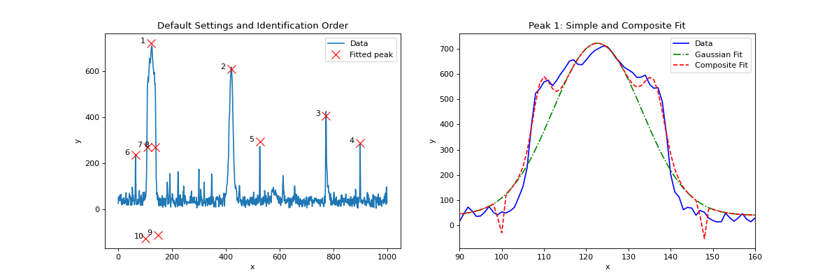
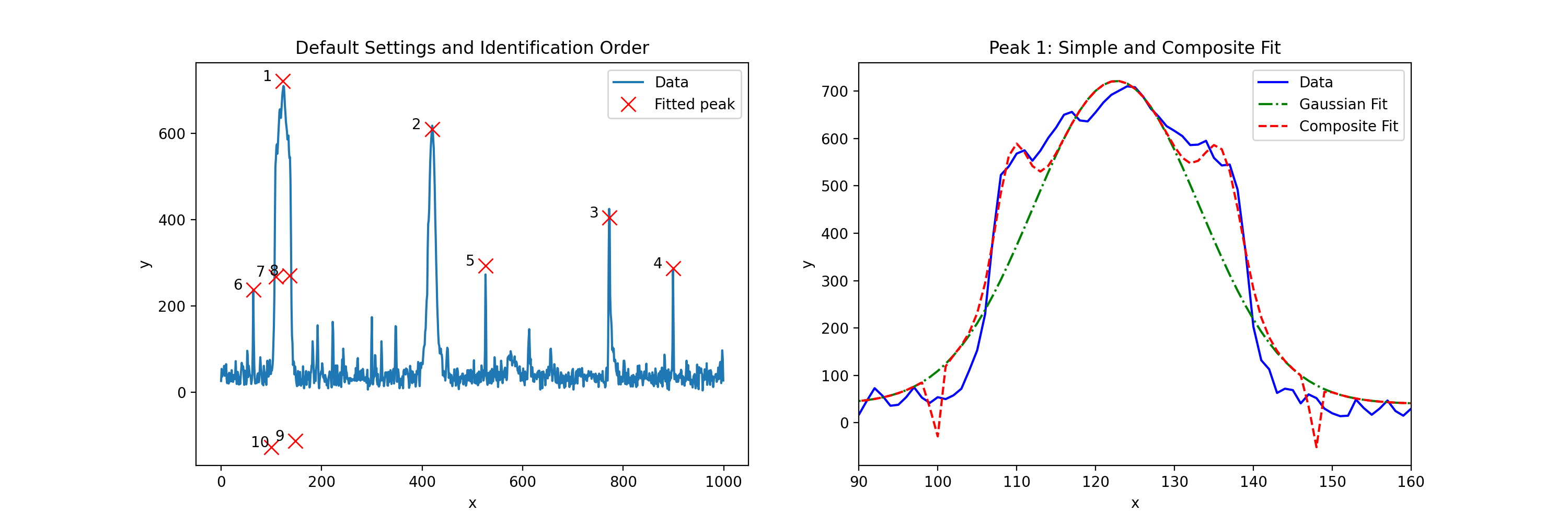
In this example, we use the default behaviour of fitpeaks1d() to identify the 10 most prominent peaks (positive and negative), in order of amplitude, from a set of data containing many possible sources. By default, fitpeaks1d() will fit Gaussian sources and with a constant background offset.

For this particular data set, attempting to identify this many peaks resulted in 4 false detections (points 7-10). This is because we are using Gaussians to model sources that do not fit such a profile. Therefore, the model has fit the most prominent source as a composite of 5 Gaussian sources as shown in the right-most plot.