The sofia_redux.toolkit.convolve.kernel module contains the ConvolveBase class, inheritors of ConvolveBase, and functional wrappers for these classes.

Convolution

Currently the following classes may be used to filter and smooth data via kernel convolution in N-dimensions:

• BoxConvolve

• KernelConvolve

• SavgolConvolve

All classes inherit from the sofia_redux.toolkit.base.Model class, shared by sofia_redux.toolkit.fitting.polynomial.Polyfit, so much of the statistical functionality and robust outlier rejection will also apply in the following section. While there are many, many algorithms available for convolution in the Python ecosystem already, the main functionality of these classes is that they allow for:

• N-dimensional

• Interpolation over masked/NaN values

• Error propagation

• Statistical analysis and outlier rejection

This is achieved using a combination of linear interpolation with Delaunay triangulation (when more than a single dimension is involved). Therefore, if none of the above features are required, it is recommended to use one of the more standard algorithms for speed by avoiding the triangulation step. Regardless, these algorithms are still quite fast.

Basic Functionality

import numpy as np
import matplotlib.pyplot as plt
import imageio
from sofia_redux.toolkit.convolve.kernel import BoxConvolve

image = imageio.imread('imageio:coffee.png').sum(axis=2)  # Gray scale
image = (image - image.min()) / (np.ptp(image))  # normalize for plotting
mean_smooth = BoxConvolve(image, 11)  # an 11 x 11 box filter

fig, ax = plt.subplots(nrows=1, ncols=2, figsize=(10, 5))
fig.tight_layout()
ax[0].imshow(image, cmap='gray')
ax[0].set_title("Original Image")
ax[1].imshow(mean_smooth.result, cmap='gray')
ax[1].set_title("Smoothed Image")

(Source code, png, hires.png, pdf)

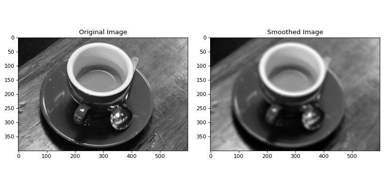
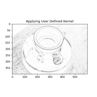
In the above example, BoxConvolve was used to set the value of each pixel to the mean value of an (11, 11) box kernel centered on each pixel. BoxConvolve is convenient, but only really just a child of KernelConvolve which does the same thing except allows the user to define their own smoothing kernel. For example, we could create a user defined Sobel filter to enhance edges in the image:

import numpy as np
import matplotlib.pyplot as plt
import imageio
from sofia_redux.toolkit.convolve.kernel import KernelConvolve

image = imageio.imread('imageio:coffee.png').sum(axis=2)  # Gray scale
image = (image - image.min()) / (np.ptp(image))  # normalize for plotting

# Create a Sobel filter
sobel = np.array([[-1, 0, 1], [-2, 0, 2], [-1, 0, 1.]])

# Edges in 1 direction
sx = KernelConvolve(image, sobel, normalize=False).result

# Edges in the other
sy = KernelConvolve(image, sobel.T, normalize=False).result

# Edge amplitude
sxy = np.hypot(sx, sy)

plt.figure(figsize=(5, 5))
plt.imshow(sxy, cmap='gray_r')
plt.title("Applying User Defined Kernel")

(Source code, png, hires.png, pdf)

Normalization

By default, a kernel (\(K\)) will be normalized before being applied to the data such that

\begin{eqnarray} & \hat{K} & = \frac{K}{\sum{K}} \\ & \sum{\hat{K}} & = 1 \end{eqnarray}

However, this will only be done if \(\sum{K} \neq 0\). To keep the original \(K\), rather the normalized kernel \(\hat{K}\), set normalize=False during initialization.

s = KernelConvolve(data, kernel, normalize=False)

Masked Values, NaN handling and Error Propagation

Missing (NaN) values and masked values (those defined by the user to ignore) are treated in the same way by the ConvolveBase class. Linear interpolation is first performed to generate values at these locations before convolution.

Errors are propagated, consistent with the initial interpolation and subsequent convolution. For 1-dimensional data, standard linear interpolation is performed. For higher dimensions, Delaunay triangulation is used instead. Therefore, one would expect 3 points used for the calculation of each interpolant in 2 dimensions, 4 points in 3-dimensions etc. This is reflected during error propagation which will be contingent on the number of points and structure of the tessellation.

In a similar way to most other classes in sofia_redux.toolkit.convolve, NaNs may be ignored (default), or propagated (ignorenans=False). Note however, that NaNs will then propagate through the convolution operation, expanding any NaN value through the entirety of the kernel. I.e., if a single NaN is present in the original data and convolved with a kernel of width 5, a NaN region of width=5 will be present in the output convolution.

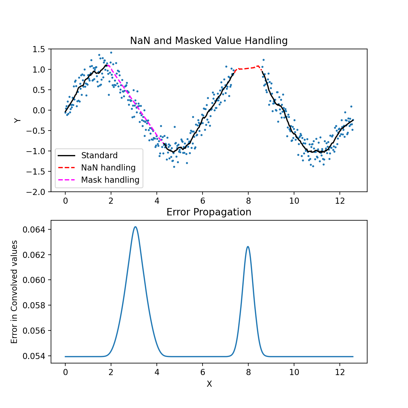
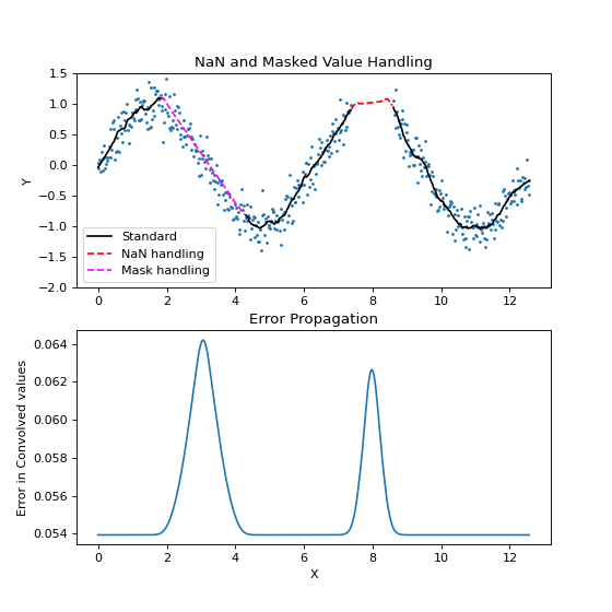
The example below uses a Savitzky-Golay filter which approximates polynomial interpolation for regularly spaced data. Large regions of the samples are set to NaN values or masked out.

import numpy as np
import matplotlib.pyplot as plt
from sofia_redux.toolkit.convolve.kernel import SavgolConvolve

x = np.linspace(0, 4 * np.pi, 512)
y = np.sin(x)
error = 0.2
rand = np.random.RandomState(41)
noise = rand.normal(loc=0.0, scale=error, size=x.size)
y += noise

# Add NaN Values
y[300:350] = np.nan

# Mask certain values to be excluded from fit, but interpolated over
mask = np.full(x.size, True)
mask[75:175] = False

width = 31
s = SavgolConvolve(x, y, width, error=error, mask=mask, order=2)

fig, ax = plt.subplots(nrows=2, ncols=1, figsize=(7, 7))
black_plot = s.result.copy()
black_plot[~mask] = np.nan
black_plot[np.isnan(y)] = np.nan
ax[0].set_title("NaN and Masked Value Handling")
ax[0].plot(x, y, '.', markersize=3)
ax[0].plot(x, black_plot, color='black',
           label='Standard')
ax[0].plot(x[300:350], s.result[300:350], '--', color='red',
           label='NaN handling')
ax[0].plot(x[75:175], s.result[75:175], '--', color='magenta',
           label='Mask handling')
ax[0].legend(loc='lower left')
ax[0].set_ylim(-2, 1.5)

ax[1].set_title("Error Propagation")
ax[1].plot(x, s.error)
ax[1].set_xlabel("X")
ax[1].set_ylabel("Error in Convolved values")
ax[0].set_ylabel("Y")

(Source code, png, hires.png, pdf)

Robust Outlier Rejection and Statistics for the Convolve Class

In a similar way to the sofia_redux.toolkit.fitting.polynomial.Polyfit class, children of Convolve may perform robust outlier rejection. An outlier is determined from the magnitude of the residual of the original data samples to the convolved values. Such outliers will be masked out and replaced with a linear interpolation from values determined to be within the rejection threshold. This process is repeated until no new outliers are found or one of the other conditions described in robust outlier rejection for sofia_redux.toolkit.fitting.polynomial.Polyfit is met.

import imageio
import numpy as np
import matplotlib.pyplot as plt
from sofia_redux.toolkit.convolve.kernel import SavgolConvolve

# Normalize for plotting
image = imageio.imread('imageio:immunohistochemistry.png').astype(float)
image = image.sum(axis=-1)
image -= image.min()
image /= image.max()

# Add some bad values
rand = np.random.RandomState(41)
inds = rand.choice(image.shape[0], 100), rand.choice(image.shape[1], 100)
image[inds] += 2

mask = np.full(image.shape, True)
mask[inds] = False

s = SavgolConvolve(image, 7, order=3)
s_robust = SavgolConvolve(image, 7, robust=5, order=3)

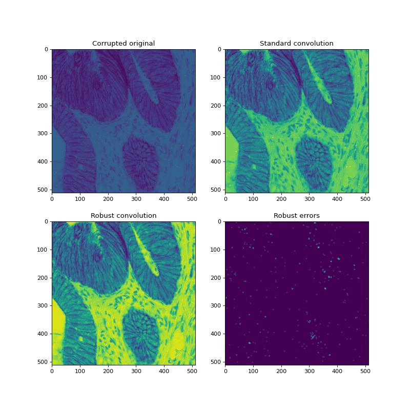
fig, ax = plt.subplots(nrows=2, ncols=2, figsize=(10, 10))
ax[0, 0].imshow(image)
ax[0, 0].set_title("Corrupted original")
ax[0, 1].imshow(s.result)
ax[0, 1].set_title("Standard convolution")
ax[1, 0].imshow(s_robust.result)
ax[1, 0].set_title("Robust convolution")
ax[1, 1].imshow(s_robust.error)
ax[1, 1].set_title("Robust errors")

# Display statistics
print(s_robust)

(Source code, png, hires.png, pdf)

Output:

Name: SavgolConvolve

         Statistics
--------------------------------
Number of original points : 262144
           Number of NaNs : 0
       Number of outliers : 420
     Number of points fit : 261724
       Degrees of freedom : 261724
              Chi-Squared : 1841.870250
      Reduced Chi-Squared : 0.007037
      Goodness-of-fit (Q) : 0.000000
     RMS deviation of fit : 0.028076
  Outlier sigma threshold : 5
  eps (delta_sigma/sigma) : 0.01
               Iterations : 3
    Iteration termination : delta_rms/rms = 0.001941

The above example shows an artificially corrupted image, the effects of convolution without removing outliers, a convolution with outliers removed, and the resulting errors from the robust convolution algorithm. Visually, all outliers have been removed.