Convolution Filters

The sofia_redux.toolkit.convolve.filter module currently contains Sobel and Savitzky-Golay filters. These are 1-dimensional filters that are applied in serial if an operation over multiple dimensions is required.

Edge Effects

Convolution at the edges of data arrays are handled according to the following rules, and may be passed into either sobel() or savgol() using the mode keyword argument as defined by scipy.signal:

‘mirror’:

Repeats the values at the edges in reverse order. The value closest to the edge is not included.

‘nearest’:

The extension contains the nearest input value.

‘constant’:

The extension contains the value given by the cval argument.

‘wrap’:

The extension contains the values from the other end of the array.

For example, if the input is [1, 2, 3, 4, 5, 6, 7, 8], and window_length is 7, the following shows the extended data for the various mode options (assuming cval is 0):

mode       |   Ext   |         Input          |   Ext
-----------+---------+------------------------+---------
'mirror'   | 4  3  2 | 1  2  3  4  5  6  7  8 | 7  6  5
'nearest'  | 1  1  1 | 1  2  3  4  5  6  7  8 | 8  8  8 (not available for savgol)
'constant' | 0  0  0 | 1  2  3  4  5  6  7  8 | 0  0  0
'wrap'     | 6  7  8 | 1  2  3  4  5  6  7  8 | 1  2  3
'reflect'  | 3  2  1 | 1  2  3  4  5  6  7  8 | 8  7  6 (not available for savgol)
'interp'   | 1  1  1 | 1  2  3  4  5  6  7  8 | 8  8  8 (not available for sobel)

The default mode for savgol() is ‘nearest’, and the default mode for sobel() is ‘reflect’.

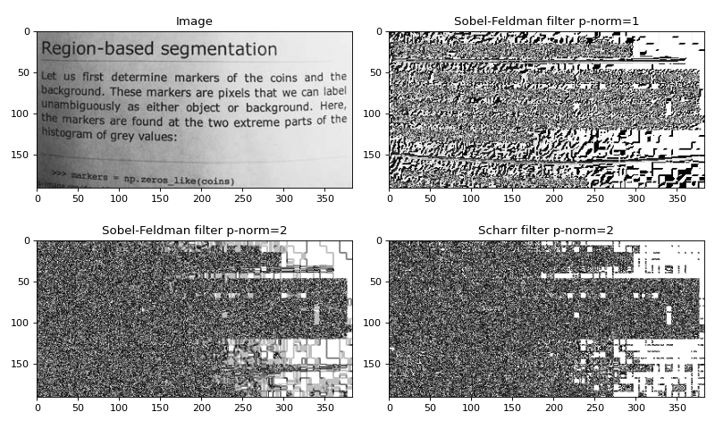
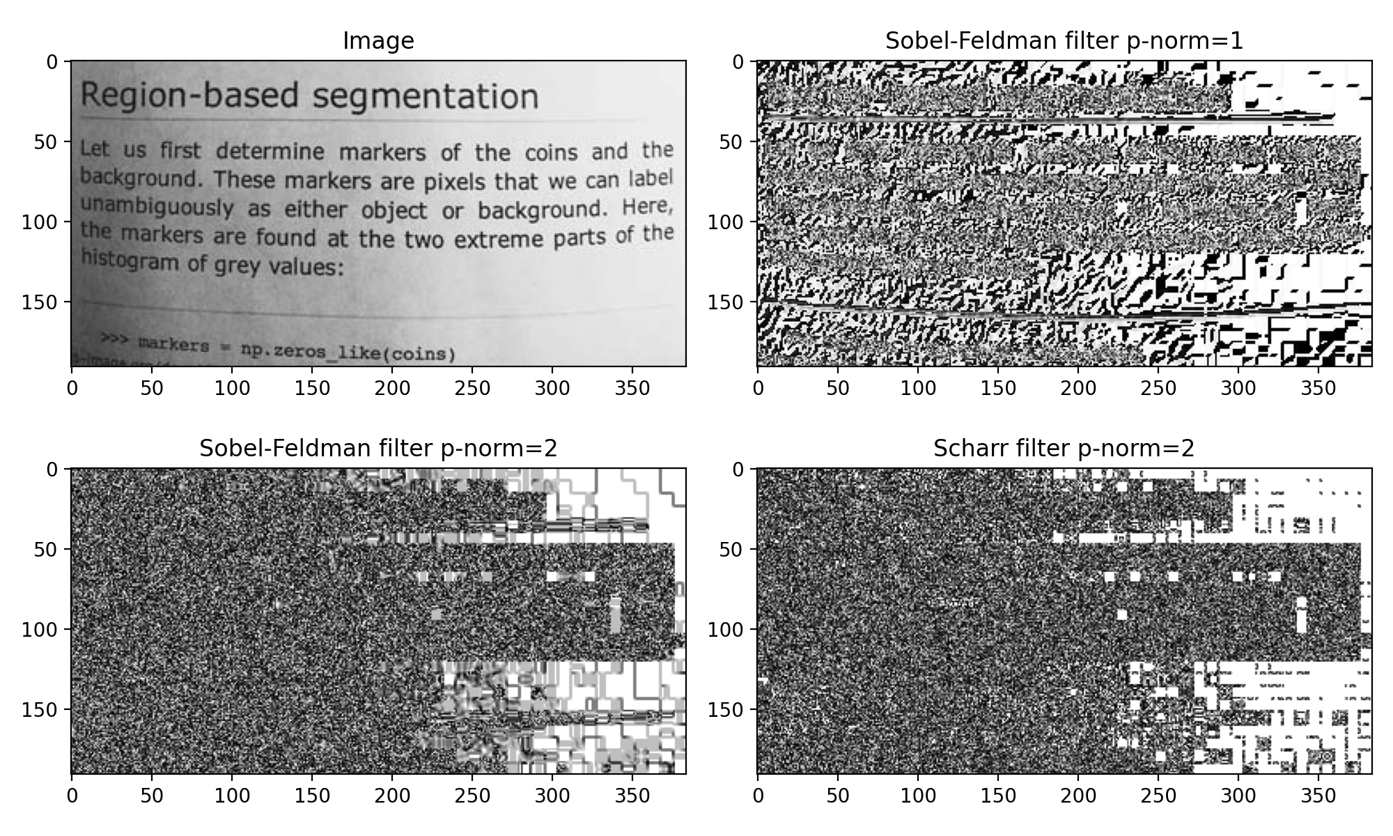
Sobel-Feldman Filtering

The Sobel-Feldman kernel is used for edge enhancement by returning an approximation to the gradient over each dimension and returning the gradient magnitude as

\[G = \|g\|_{2} = \sqrt{\sum_{i=1}^{N}{g_{i}^{2}}}\]

However, sobel() was designed to replicate the IDL implementation of the Sobel-Feldman filter in the sobel function, which only operates on 2-dimensional data, and also defines the gradient magnitude as:

\[G = \|g\|_{1} = | g_{x} | + | g_{y} |\]

I.e., the general implementation uses the Euclidean norm, while IDL uses the Manhattan norm. Therefore, sobel() allows for a p-norm implementation with a default of \(p=1\). The p-norm returns a value such that

\[G = \| g \|_{p} = \left(\sum_{i=1}^{N}{| g_i |^{p}}\right)^\frac{1}{p}\]

An estimate of the gradient \(g_i\) for dimension \(i\) is given by applying a kernel that is the result of two separable functions. For the Sobel-Feldman filter these are:

• Derivative direction: \(h(-1)=-1, h(0)=0, h(1)=1\)

• Perpendicular to derivative direction: \(h^{\prime}(-1)=1, h^{\prime}(0)=2, h^{\prime}(1)=1\)

For example, in 2-dimensions:

\begin{eqnarray} g_{x} &= & \begin{bmatrix} -1 & 0 & +1 \\ -2 & 0 & +2 \\ -1 & 0 & +1 \end{bmatrix} \circledast d \\ g_{y} &= & \begin{bmatrix} -1 & -2 & -1 \\ 0 & 0 & 0 \\ +1 & +2 & +1 \end{bmatrix} \circledast d \end{eqnarray}

The filter used can be defined using the kderiv and kperp keyword argument. By default, these are set to kderiv=(-1, 0, 1) and kperp=(1, 2, 1) in order to produce a Sobel-Feldman filter. However, there is no reason that different filter values or even different sizes cannot be provided.

import matplotlib.pyplot as plt
import imageio
from sofia_redux.toolkit.convolve.filter import sobel

image = imageio.imread('imageio:page.png')
fig, ax = plt.subplots(nrows=2, ncols=2, figsize=(10, 6))
ax[0, 0].imshow(image, cmap='gray')
ax[0, 0].set_title("Image")
ax[0, 1].imshow(sobel(image), cmap='gray_r')
ax[0, 1].set_title("Sobel-Feldman filter p-norm=1")
ax[1, 0].imshow(sobel(image, pnorm=2), cmap='gray_r')
ax[1, 0].set_title("Sobel-Feldman filter p-norm=2")
ax[1, 1].imshow(sobel(image, pnorm=2, kperp=(3, 10, 3)), cmap='gray_r')
ax[1, 1].set_title("Scharr filter p-norm=2")
fig.tight_layout()

(Source code, png, hires.png, pdf)

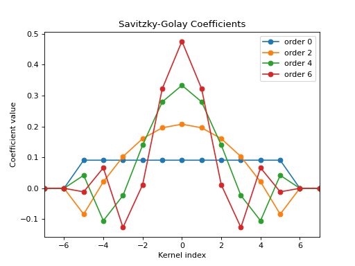
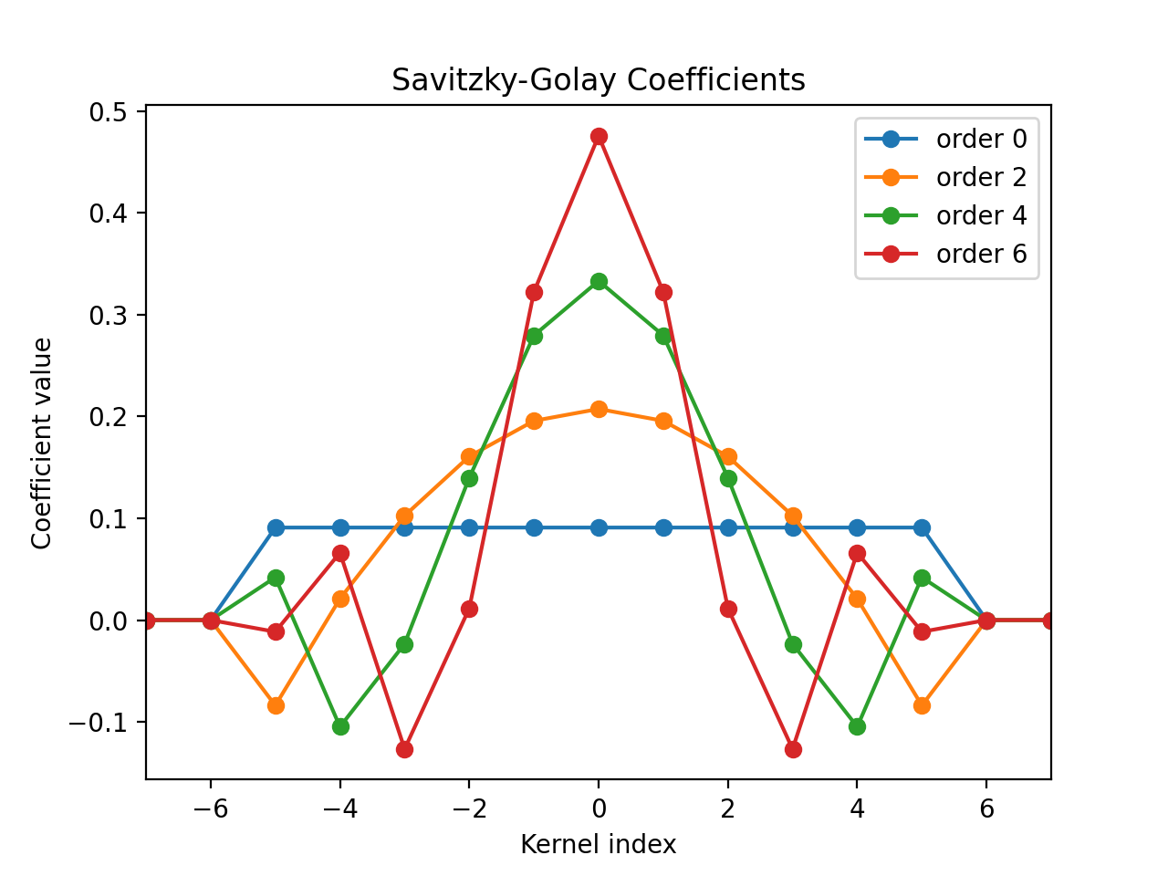
Savitzky-Golay Filter

The savgol() function is used to create the Savitzky-Golay filter and apply filtering over N-dimensions. Convolution with the Savitzky-Golay filter essentially fits a polynomial of a given order using linear least squares so long as data points are equally spaced.

The user must pass in a window argument specifying the width of the filtering window over each dimension (may be a single value for each dimension, or an array containing the window width for each dimension). The default polynomial order is 2 for each dimension, but may also be specified for all, or per dimension, using order. The following displays the various orders of the 1-dimensional Savitzky-Golay filter for a window of width 11:

import numpy as np
import matplotlib.pyplot as plt
from sofia_redux.toolkit.convolve.filter import savgol

x = np.arange(-20, 20)
y = np.zeros(x.size)
y[x.size // 2] = 1

for i in range(0, 8, 2):
    plt.plot(x, savgol(y, 11, order=i), '-o', label="order %i" % i)
plt.legend()
plt.xlim(-7, 7)
plt.title("Savitzky-Golay Coefficients")
plt.xlabel("Kernel index")
plt.ylabel("Coefficient value")

(Source code, png, hires.png, pdf)

Be aware that the Savitzky-Golay coefficients are generated as a function of \(\lfloor\frac{order}{2}\rfloor\) so that orders 0 and 1 produce the same results, as do orders 2 and 3, etc.

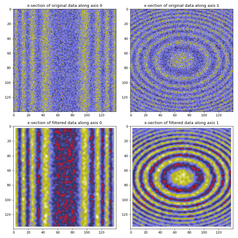
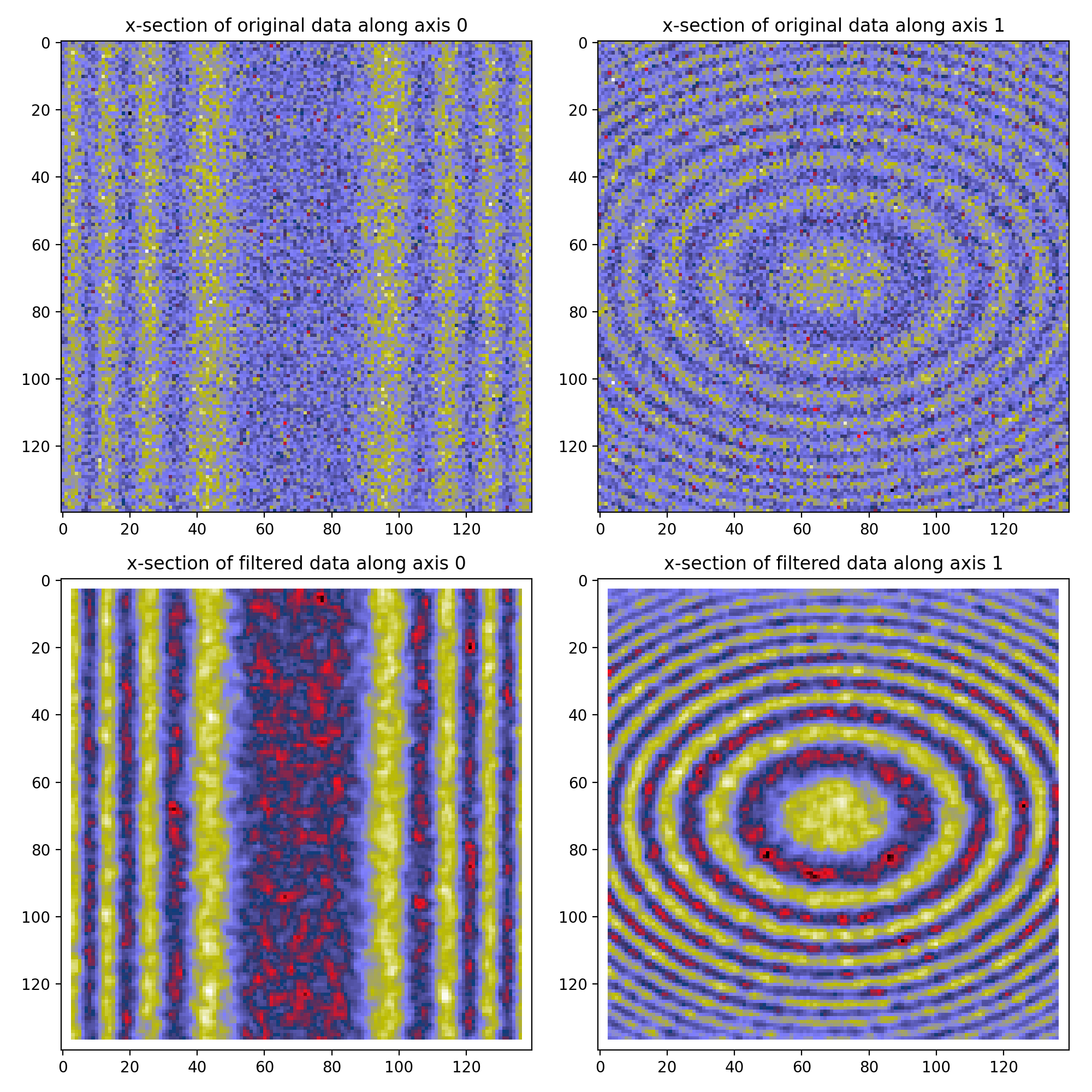
The following example applies a 2nd order Savitzky-Golay filter of width 7 to a 3-dimensional data set.

import numpy as np
import matplotlib.pyplot as plt
from sofia_redux.toolkit.convolve.filter import savgol

x, y, z = np.mgrid[-70:70, -70:70, -70:70]
d = np.cos((x ** 2 + x ** 2 + z ** 2) / 200)
rand = np.random.RandomState(41)
d += rand.normal(size=x.shape)

result = savgol(d, 7, order=2, mode='constant', cval=np.nan)
fig, ax = plt.subplots(nrows=2, ncols=2, figsize=(10, 10))
c = 'gist_stern'
ax[0, 0].set_title("x-section of original data along axis 0")
ax[0, 0].imshow(d[40], cmap=c)
ax[0, 1].set_title("x-section of original data along axis 1")
ax[0, 1].imshow(d[:, 40], cmap=c)
ax[1, 0].set_title("x-section of filtered data along axis 0")
ax[1, 0].imshow(result[40], cmap=c)
ax[1, 1].set_title("x-section of filtered data along axis 1")
ax[1, 1].imshow(result[:, 40], cmap=c)
fig.tight_layout()

(Source code, png, hires.png, pdf)

Note that a NaN border has been placed around the filtered image using mode='constant, cval=np.nan. The sofia_redux.toolkit.convolve.kernel.SavgolConvolve class and sofia_redux.toolkit.convolve.kernel.savitzky_golay() function are wrappers for the savgol() function, but allow the additional functionality of NaN handling, robust outlier rejection, statistics, and error propagation.