HAWC+ DRP Developer’s Manual#

Introduction#

Document Purpose#

This document is intended to provide all the information necessary to maintain the HAWC+ DRP pipeline, used to produce Level 2, 3, and 4 reduced products for HAWC+ data, in either manual or automatic mode. Level 2 is defined as data that has been processed to correct for instrumental effects; Level 3 is defined as data that has been flux-calibrated. Level 4 is any higher-level data product. A more general introduction to the data reduction procedure and the scientific justification of the algorithms is available in the HAWC+ DRP Users Manual.

This manual applies to HAWC+ DRP version 3.2.0.

HAWC DRP Revision History#

The HAWC pipeline was originally developed as three separate packages: the HAWC Data Reduction Pipeline (DRP), which contains pipeline infrastructure and chop/nod imaging and polarimetry reduction algorithms; the Comprehensive Reduction Utility for SHARC-2 (CRUSH), which contained scan-mode data reduction algorithms; and Redux, which provides the interface to the pipeline algorithms for command-line and interactive use.

The HAWC DRP was developed by the HAWC+ team at Northwestern University and University of Chicago, principally Dr. Marc Berthoud, Dr. Fabio Santos, and Dr. Nicholas Chapman, under the direction of the HAWC+ Principal Investigator, Dr. C. Darren Dowell, and the software lead, Dr. Giles Novak. The DRP infrastructure has roots in an earlier data reduction pipeline, built for SOFIA’s FORCAST instrument, while many of the scientific algorithms were originally developed for SHARC-2/SHARP, the Caltech Submillimeter Observatory’s imaging polarimeter.

CRUSH began as a PhD project at Caltech to support data reduction for the SHARC-2 instrument, but has since been expanded to support data reduction for many other instruments. It was originally developed and maintained by Dr. Attila Kovács.

The SOFIA Data Processing Systems (DPS) team provided the Redux interface package and develops, maintains, integrates, and releases the HAWC pipeline. DPS first released the pipeline for SOFIA data reductions in January 2017. Starting January 2019, the DPS also maintained a local fork of the CRUSH pipeline, for further development and support of the scan-mode algorithms. In addition, as of HAWC DRP v2.1.0, some calibration and general data reduction utilities were moved to packages shared by other SOFIA pipelines (sofia_redux.calibration and sofia_redux.toolkit, respectively).

In 2020, all SOFIA pipeline packages were unified into a single package, called sofia_redux. The interface package (Redux) was renamed to sofia_redux.pipeline, and the HAWC DRP package was renamed to sofia_redux.instruments.hawc.

In 2022, the Java implementation of the CRUSH pipeline was replaced by a Python implementation in the SOFIA Redux package, at sofia_redux.scan.

Overview of Software Structure#

The sofia_redux package has several sub-modules organized by functionality:

sofia_redux
├── calibration
├── instruments
│   ├── exes
│   ├── fifi_ls
│   ├── flitecam
│   ├── forcast
│   └── hawc
├── pipeline
├── scan
├── spectroscopy
├── toolkit
└── visualization

The modules used in the HAWC pipeline are described below.

DRP Architecture#

The HAWC DRP (sofia_redux.instruments.hawc) package is written in Python using standard scientific tools and libraries. It has two main structures: data containers and the data processing algorithms (pipe steps).

In the DRP, data reduction proceeds by creating and calling pipeline Step objects, each of which is responsible for a single step in the data reduction. Pipe steps (e.g. StepPrepare, StepDemodulate, etc.) inherit from StepParent objects that define how a step is executed on its inputs, and how its outputs are returned. Input and output data are stored and exchanged in Data objects. Typically, these Data objects contain the equivalent of a FITS file (DataFits), with a header structure and binary data arranged into header-data units (HDUs), but may optionally correspond to a text file (DataText) or other format. All pipeline components use a common configuration object and send messages to common logger objects. See Fig. 131 for a class diagram of the relationships between the most important DRP classes.

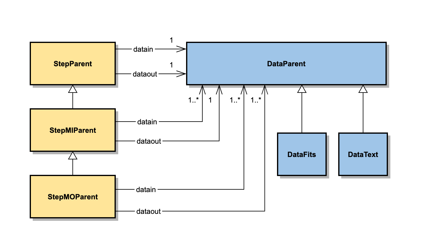
Fig. 131 DRP Core Class Diagram. Pipeline steps inherit from StepParent (for single-input, single-output steps), StepMIParent (for multi-input, single-output steps) or from StepMOParent (for multi-input, multi-output steps). Input and output data for the steps may be any object that inherits from DataParent, but are typically DataFits objects.#

Data Objects#

The pipeline data objects, which inherit from DataParent, store raw, partly-reduced, or fully-reduced data. This structure is used for both the FITS files saved to disk as well as the data in memory that is passed between pipeline steps. The most commonly used object, DataFits, stores data as astropy.io.fits header-data units (HDUs). It can load, copy, or store image HDUs or binary table HDUs, in addition to the primary HDU. The primary extension typically contains the image data that is most important to the user. All secondary images and tables store additional information (noise, exposure maps, bad pixel maps, etc.), each with a unique EXTNAME stored in their associated headers. Images may be accessed with the DataFits.imageget(), DataFits.imageset(), and DataFits.imagedel() methods. Tables can be accessed with DataFits.tableget(), DataFits.tableset(), and DataFits.tabledel() methods. DataFits also has table manipulation methods that can be used to modify a table extension in place (DataFits.tableaddcol(), DataFits.tablemergerows(), etc.).

The primary header typically contains the same keywords as the raw input data. In addition, each pipeline step adds a HISTORY keyword to the FITS header and updates the PRODNAME, PROCSTAT, and PIPEVERS keywords. When input files are merged in multi-input, single-output steps, most keywords are taken from the first input header, but some keywords may require special handling (averaging, concatenation, or other operations across the input set). These special merge handling procedures are specified in the DRP configuration file, in the [headmerge] section, and are handled by the DataFits.mergehead() method.

Header keywords may also be overridden in the configuration file, in the [header] section. When the DataFits.getheadval() method is called, it first checks the configuration file for a keyword in this section. If it is found, it is used instead of the value from the stored header. For this reason, it is recommended to retrieve all FITS keywords with the getheadval method, rather than accessing DataFits.header directly. FITS keywords should also be set with the setheadval method.

Pipeline data objects also store their own file names. Pipeline steps update the file name in the object before returning them as output, using the filenamebegin, filenameend, and filenum keywords in the [data] section of the configuration file to determine how to insert the product type (a three-letter identifier, different for each pipeline step) and compose a new output name. The file name segments for any data object can be accessed by calling DataFits.filename for the full name (including path), DataFits.filenamebegin for all parts of the name up to the product type, DataFits.filenameend for all parts of the name after the product type, and DataFits.filenum for the file number embedded in the file name.

Pipeline data objects also store a configuration object in ConfigObj format and a logging object for passing messages to. See Fig. 132 for brief documentation of the most important attributes and operations of the DataFits object.

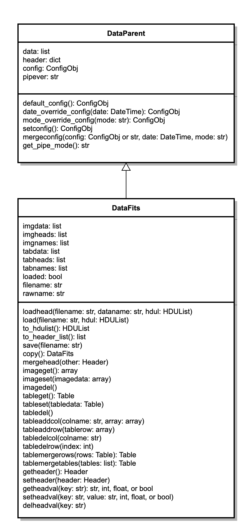
UML class diagram for DataFits. — Fig. 132 DataFits class diagram.#

Pipeline Steps#

The pipeline step objects contain the main function for a single data reduction algorithm, along with its associated parameters. Each step object is directly callable as, for example,

intermediate = StepOne(input)

where input is generally a list of DataFits objects containing the data to operate on, and intermediate is a list of output DataFits objects, on which the operation has been performed.

All pipeline steps inherit from a common parent object (StepParent) or one of its children (StepMIParent, StepMOParent). Most pipe steps are single-input, single-output (SISO) steps, which inherit directly from StepParent. That is, they take a single Data object as input and return a single Data object as output. They may be called in a loop to process a series of files at once. Some steps may implement algorithms that operate on a list of Data objects and return a single Data object as output (multi-input, single output; MISO). These inherit from StepMIParent. Some steps may also operate on a list of Data objects at once, but still return multiple output files (multi-input, multi-output; MIMO). These inherit from StepMOParent. See Fig. 133 for a diagram of the Step parent classes.

Parameters for each step are generally defined in their setup method. Each parameter is a list containing the parameter name, default value, and a comment. Parameters for the step are stored in a list in the paramlist attribute, and may be retrieved by calling the StepParent.getarg() method. This method first checks for a value in a configuration file; if not found, the default value will be used.

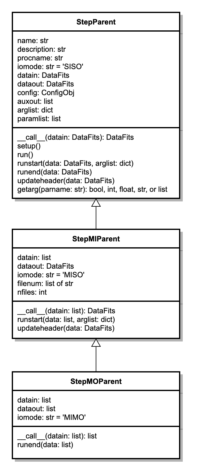
StepParent Class Diagram. — Fig. 133 StepParent class diagram.#

Scan Map Architecture#

The scan package (sofia_redux.scan) package implements an iterative map reconstruction algorithm, for reducing continuously scanned observations. It is implemented in pure Python, with numba just-in-time (JIT) compilation support for heavy numerical processes, and multiprocessing support for parallelizable loops.

Class Relationships#

Main Classes#

The primary data structures for modeling an instrument in the scan package are listed below, and their relationships are diagrammed in Fig. 8.

ChannelData: an class representing a set of detector channel (pixels). A channel has properties, such as gains, flags, and weights etc.
ChannelGroup: A generic grouping of detector channels. This is implemented as a wrapper around the ChannelData class, with access to specific channel indices held by the underlying arrays.
Channels: An class representing all the available channels for an instrument.
Frames: A data structure that represents the readout values of all Channels at a given time sample, together with software flags, and associated properties (e.g. gain, transmission, weight etc.)
Integration: A collection of Frames that comprises a contiguous dataset, for which one can assume overall stability of gains and noise properties. Typically an Integration is a few minutes of data.
Scan: A collection of Integrations that comprise a single file or observing entity. For HAWC+, a scan is a data file, and by default each scan contains just one integration. However, it is possible to break Scans into multiple Integrations, if desired.
Signal: An object representing some time-variant scalar signal that may (or may not) produce a response in the detector channels. For example, the chopper motion in the ‘x’ direction is such a Signal (available as ‘chopper-x’) that may be used during the reduction.
Dependents: An object that keeps track of the number of model parameters derived from each Frame and each Channel. It measures the lost degrees of freedom due to modeling (and filtering) of the raw signals, and it is critical for calculating proper noise weights that remain stable in a iterated framework. Failure to count Dependents correctly and accurately can result in divergent weighting, which in turn manifests in over-flagging and/or severe mapping artifacts. Every modeling step keeps track of its own dependents this way in the analysis.
ChannelDivision: A collection of ChannelGroups according to some grouping principle. For example, the channels that are read out through a particular SQUID multiplexer (MUX) comprise a ChannelGroup for that particular SQUID. The collection of MUX groups over all the SQUID MUXes constitute a ChannelDivision.
Mode: An object that represents how a ChannelGroup responds to a Signal.
Modality: A collection of Modes of a common type. Just as Modes are inherently linked to a ChannelGroup, Modalities are linked to ChannelDivisions.

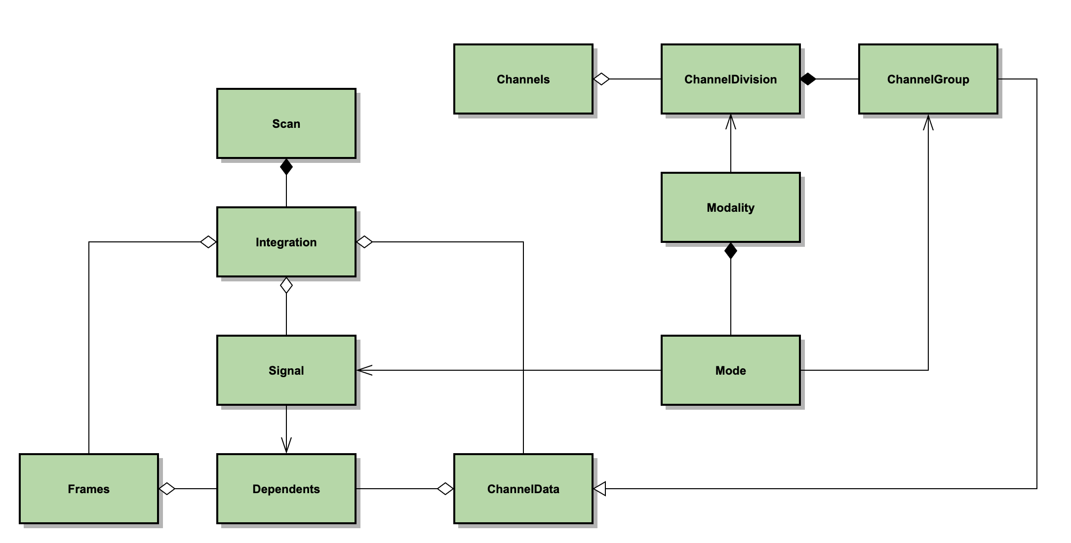
UML class diagram of principal scan data classes. — Fig. 134 Principal scan data classes. Channels has a set of ChannelDivisions. ChannelDivision is composed of ChannelGroups, which inherit from ChannelData. Modality depends on ChannelDivision and is composed of Modes. Mode depends on ChannelGroup and depends on Signal. Scan is composed of Integrations. Integration has a collection of Frames, Signals, and ChannelData. Frame and ChannelData have a collection of Dependents; Signal depends on Dependents.#

For example, the HAWC instrument is modeled as a set of Channels, i.e. pixels, for which each has a row and a column index within a subarray. The raw timestream of data from the channels is modeled as a set of Frames, contained within an Integration. To decorrelate the rows of the HAWC detector, a Modality is created from “rows” ChannelDivision. This modality contains Modes generated for each ChannelGroup with a particular row index (row=0, row=1, etc.). Each mode is associated with a Signal, which contains the correlated signals for the row, determines and updates gain increments, subtracts them from the time samples in the Frames, and updates the dependents associated with the Frames and ChannelData.

The reduction process is run from the class Reduction, which performs the reduction in a Pipeline instance, and produces a SourceModel (see Fig. 9). A Reduction may create a set of sub-reductions to run in parallel, for processing a group of separate but associated source models. These sub-reductions are used, for example, to process HAWC+ R and T subarrays separately for Scan-Pol data.

Each Pipeline is in charge of reducing a group of Scans mostly independently (apart from resulting in a combined SourceModel). The Pipeline iteratively reduces each Scan by repeatedly executing a set of tasks, defined by a Configuration class. Metadata for the observation, including the Configuration and instrument information, is managed by an Info class associated with the Reduction.

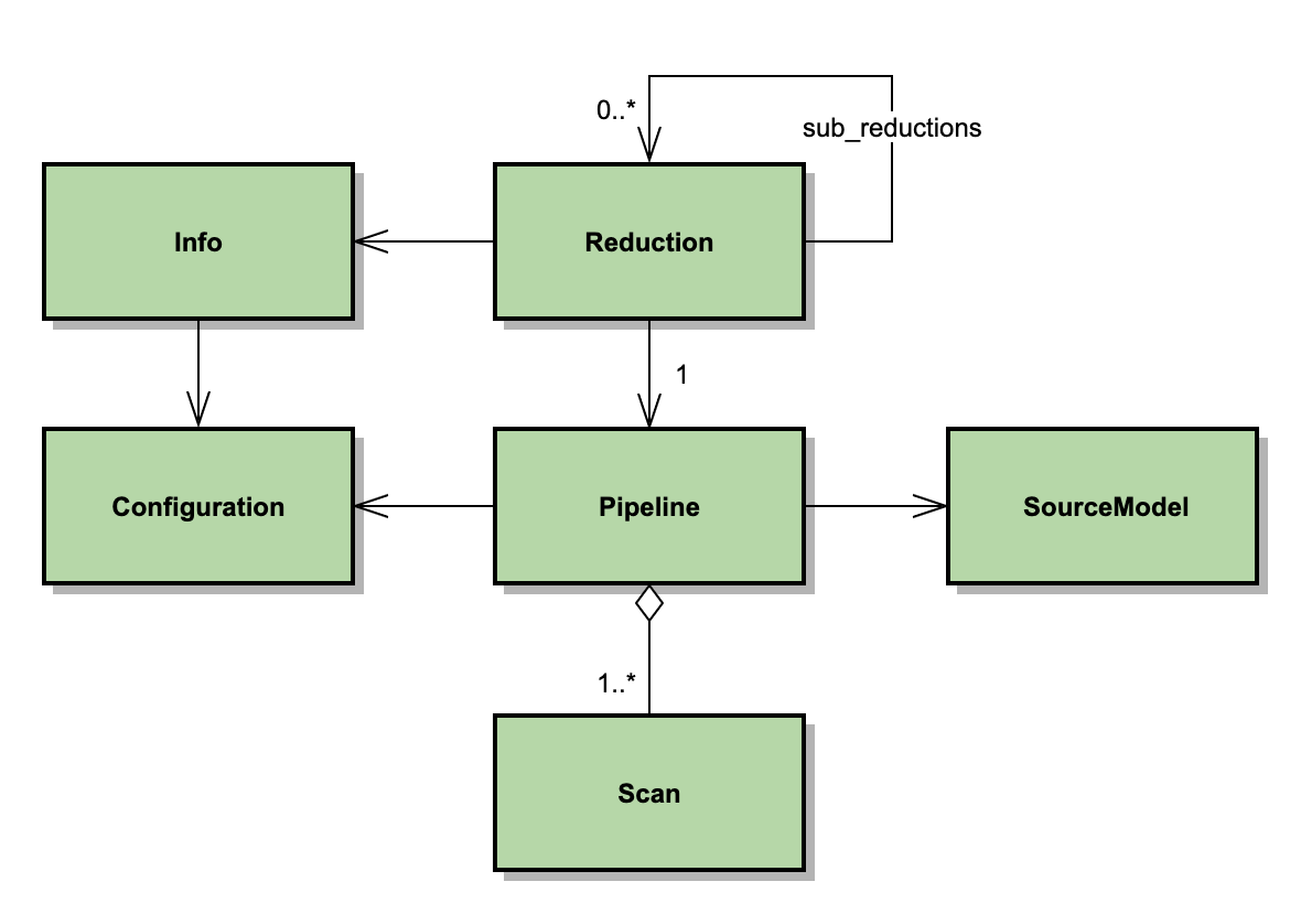
UML class diagram of principal scan processing classes. — Fig. 135 Principal scan processing classes. A Reduction creates a Pipeline or, optionally, sub-reductions that create their own Pipelines. The Reduction depends on Info, which contains a Configuration. Pipeline depends on Configuration and on SourceModel, and has an aggregation of Scans to reduce.#

HAWC+ Specific Classes#

The HAWC+ classes are derived from the above classes via a set of general SOFIA classes and several more generic classes, as listed below, and shown in Fig. 136.

HawcPlusChannelData \(\rightarrow\) SofiaChannelData \(\rightarrow\) ColorArrangementData \(\rightarrow\) ChannelData
HawcPlusChannelGroup \(\rightarrow\) ChannelGroup
HawcPlusChannels \(\rightarrow\) SofiaCamera \(\rightarrow\) SingleColorArrangement \(\rightarrow\) ColorArrangement \(\rightarrow\) Camera \(\rightarrow\) Channels
HawcPlusFrames \(\rightarrow\) SofiaFrames \(\rightarrow\) HorizontalFrames \(\rightarrow\) Frames
HawcPlusIntegration \(\rightarrow\) SofiaIntegration \(\rightarrow\) Integration
HawcPlusScan \(\rightarrow\) SofiaScan \(\rightarrow\) Scan
HawcPlusInfo \(\rightarrow\) SofiaInfo \(\rightarrow\) CameraInfo \(\rightarrow\) Info

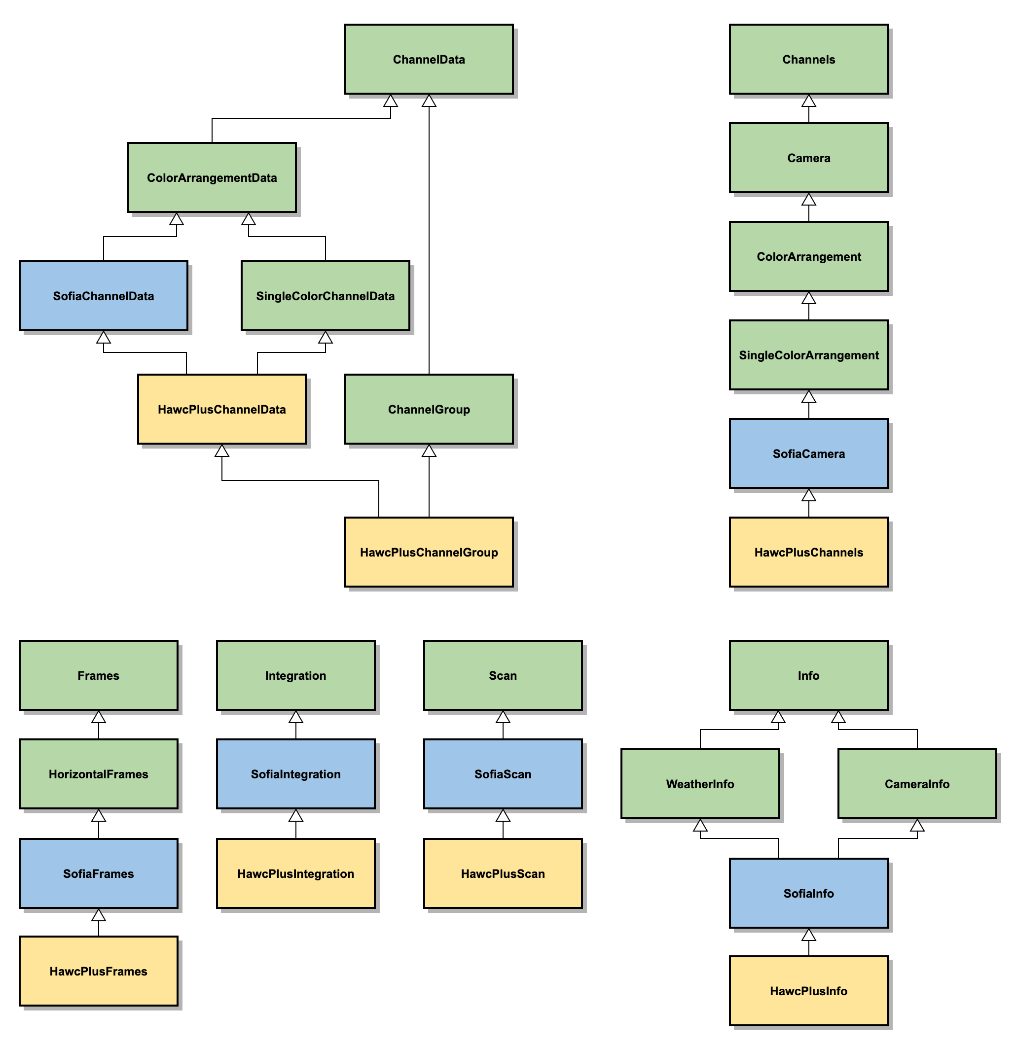
UML class diagram of HAWC+ scan classes — Fig. 136 HAWC+ specific scan classes. HAWC classes (yellow) generally inherit from SOFIA classes (blue), which inherit from more generic classes (green).#

Top-Level Call Sequence#

The symbol \(\circlearrowright\) indicates a loop, \(\pitchfork\) (fork) indicates a parallel processing fork, square brackets are methods that are called optionally (based on the current configuration settings). Only the most relevant calls are shown. Ellipses (…) are used to indicate that the call sequence may contain additional elements not explicitly listed here and/or added by the particular subclass implementations.

Call sequence from sofia_redux.scan.reduction.Reduction:

Reduction.__init__()
1. Info.instance_from_intrument_name()
2. Info.read_configuration()
3. Info.get_channels_instance()
Reduction.run()
1. Info.split_reduction()
2. \(\pitchfork\) Channels.read_scan()
  1. Channels.get_scan_instance()
  2. Scan.read(filename: str)
  3. Scan.validate()
    1. \(\circlearrowright\) Integration.validate() …
      1. Frames.validate() …
      2. \([\) Integration.fill_gaps() \(]\)
      3. \([\) Integration.notch_filter() \(]\)
      4. \([\) Integration.detect_chopper() \(]\)
      5. \([\) Integration.select_frames() \(]\)
      6. \([\) Integration.velocity_clip() / acceleration_clip() \(]\)
      7. \([\) KillFilter.apply() \(]\)
      8. \([\) Integration.check_range() \(]\)
      9. \([\) Integration.downsample() \(]\)
      10. Integration.trim()
      11. Integration.detector_stage()
      12. \([\) Integration.set_tau() \(]\)
      13. \([\) Integration.set_scaling() \(]\)
      14. \([\) Integration.slim() \(]\)
        
        Channels.slim()
        
        Frames.slim()
      15. \([\) \(\circlearrowright\) Frame.jackknife() \(]\)
      16. Integration.bootstrap_weights()
    2. Channels.calculate_overlaps()
3. Reduction.validate()
  1. Info.validate_scans()
  2. Reduction.init_source_model()
  3. Reduction.init_pipelines()
4. \(\pitchfork\) Reduction.reduce()
  1. \(\circlearrowright\) Reduction.iterate()
    1. Pipeline.set_ordering()
    2. \(\pitchfork\) Pipeline.iterate()
      1. \(\circlearrowright\) Scan.perform(task: str)
        
        \(\circlearrowright\) Integration.perform(task: str)
        
        \([\) Integration.dejump() \(]\)
        
        \([\) Integration.remove_offsets() \(]\)
        
        \([\) Integration.remove_drifts() \(]\)
        
        \([\) Integration.decorrelate(modality, …) \(]\)
        
        \([\) Integration.get_channel_weights() \(]\)
        
        \([\) Integration.get_time_weights() \(]\)
        
        \([\) Integration.despike() \(]\)
        
        \([\) Integration.filter.apply() \(]\)
      2. \(\circlearrowright\) Pipeline.update_source(Scan)
        
        SourceModel.renew()
        
        \(\circlearrowright\) SourceModel.add_integration(Integration)
        
        SourceModel.process_scan(Scan) …
        
        SourceModel.add_model(SourceModel)
        
        SourceModel.post_process_scan(Scan)
  2. \([\) Reduction.write_products() \(]\)

Most of the number crunching happens under the Integration.perform call, highlighted in bold-face. It is a switch method that will make the relevant processing calls, in the sequence defined by the current pipeline configuration.

Redux Architecture#

Design#

Redux is designed to be a light-weight interface to data reduction pipelines. It contains the definitions of how reduction algorithms should be called for any given instrument, mode, or pipeline, in either a command-line interface (CLI) or graphical user interface (GUI) mode, but it does not contain the reduction algorithms themselves.

Redux is organized around the principle that any data reduction procedure can be accomplished by running a linear sequence of data reduction steps. It relies on a Reduction class that defines what these steps are and in which order they should be run (the reduction “recipe”). Reductions have an associated Parameter class that defines what parameters the steps may accept. Because reduction classes share common interaction methods, they can be instantiated and called from a completely generic front-end GUI, which provides the capability to load in raw data files, and then:

set the parameters for a reduction step,
run the step on all input data,
display the results of the processing,

and repeat this process for every step in sequence to complete the reduction on the loaded data. In order to choose the correct reduction object for a given data set, the interface uses a Chooser class, which reads header information from loaded input files and uses it to decide which reduction object to instantiate and return.

The GUI is a PyQt application, based around the Application class. Because the GUI operations are completely separate from the reduction operations, the automatic pipeline script is simply a wrapper around a reduction object: the Pipe class uses the Chooser to instantiate the Reduction, then calls its reduce method, which calls each reduction step in order and reports any output files generated. Both the Application and Pipe classes inherit from a common Interface class that holds reduction objects and defines the methods for interacting with them. The Application class additionally may start and update custom data viewers associated with the data reduction; these should inherit from the Redux Viewer class.

All reduction classes inherit from the generic Reduction class, which defines the common interface for all reductions: how parameters are initialized and modified, how each step is called. Each specific reduction class must then define each data reduction step as a method that calls the appropriate algorithm.

The reduction methods may contain any code necessary to accomplish the data reduction step. Typically, a reduction method will contain code to fetch the parameters for the method from the object’s associated Parameters class, then will call an external data reduction algorithm with appropriate parameter values, and store the results in the ‘input’ attribute to be available for the next processing step. If processing results in data that can be displayed, it should be placed in the ‘display_data’ attribute, in a format that can be recognized by the associated Viewers. The Redux GUI checks this attribute at the end of each data reduction step and displays the contents via the Viewer’s ‘display’ method.

Parameters for data reduction are stored as a list of ParameterSet objects, one for each reduction step. Parameter sets contain the key, value, data type, and widget type information for every parameter. A Parameters class may generate these parameter sets by defining a default dictionary that associates step names with parameter lists that define these values. This dictionary may be defined directly in the Parameters class, or may be read in from an external configuration file or software package, as appropriate for the reduction.

HAWC Redux#

To interface to the HAWC DRP pipeline, Redux defines the HAWCReduction and HAWCParameters classes. See Fig. 137 for a sketch of the Redux classes used by the HAWC pipeline. The HAWCReduction class holds the DRP DataFits objects and calls the DRP Step classes. The HAWCParameters class reads from the DRP configuration object.

The HAWCParameters class uses the DRP configuration file to define all parameters for DRP steps. Additionally, it adds a set of control parameters that the HAWCReduction class uses to determine if the output of a reduction step should be saved or displayed after processing.

The HAWCReduction class also uses the DRP configuration file to determine pipeline modes and data processing recipes for all input files. Instead of implementing a method for each reduction step, it calls a single method for each step: the run_drp_step method looks up the appropriate DRP Step class from the pipeline step name, and calls it on the data in the input attribute.

Since raw HAWC data is very large, Redux defines some of the initial data reduction steps as a combination of several DRP steps. This allows one raw file to be loaded into memory at a time, and only the smaller intermediate products to be passed along to the next reduction step. These pipeline step overrides are defined in a constant called STEPLISTS, in the HAWCParameters class. The super-step methods are defined as make_flats and demodulate methods in the HAWCReduction class.

HAWC data is displayed in the DS9 FITS viewer after each step, via the QADViewer class provided by the Redux package.

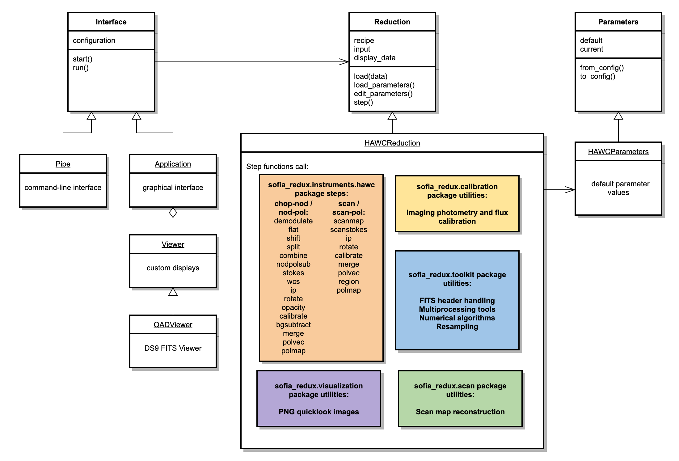
HAWC Redux Classes — Fig. 137 Redux classes used in the HAWC pipeline.#

Class Inheritance Diagram#

sofia_redux.instruments.hawc.steps.basehawc Module#

Functions#

`calchilo`(chop, nsamp, choptol, good)	Tag data as high, low, or bad.
`readchop`(step, nsamp, chop_tol[, chopflag])	Read chop state into high, low, or not used values.
`readnod`(step, nsamp, nod_tol[, nodflag])	Read nod state into high, low, or not used values.
`readhwp`(step, nsamp, hwp_tol, sampfreq)	Determine HWP state for all samples.
`clipped_mean`(data, mask[, sigma])	Compute a sigma-clipped mean of the input data.

sofia_redux.instruments.hawc.steps.basemap Module#

Classes#

BaseMap()

Functions#

pipecal_applyphot(fitsfile[, srcpos, ...])

Calculate photometry on a FITS image and store results to FITS header.

sofia_redux.calibration.pipecal_calfac Module#

Functions#

pipecal_calfac(flux, flux_err, config)

Calculate the calibration factor for a flux standard.

sofia_redux.calibration.pipecal_config Module#

Functions#

`pipecal_config`(header)	Parse all reference files and return appropriate configuration values.
`read_respfile`(fname, spectel)	Read response files.

sofia_redux.calibration.pipecal_fitpeak Module#

Functions#

`elliptical_gaussian`(coords[, baseline, ...])	Function for an elliptical Gaussian profile.
`elliptical_lorentzian`(coords[, baseline, ...])	Function for an elliptical Lorentzian profile.
`elliptical_moffat`(coords[, baseline, dpeak, ...])	Function for an elliptical Moffat profile.
`pipecal_fitpeak`(image[, profile, estimates, ...])	Fit a peak profile to a 2D image.

sofia_redux.calibration.pipecal_photometry Module#

Functions#

pipecal_photometry(image, variance[, ...])

Perform aperture photometry and profile fits on image data.

sofia_redux.calibration.pipecal_rratio Module#

Functions#

pipecal_rratio(za, altwv, za_ref, altwv_ref, ...)

Calculate the R ratio for a given ZA and Altitude or PWV.

sofia_redux.calibration.pipecal_util Module#

Functions#

`average_za`(header)	Robust average of zenith angle from FITS header.
`average_alt`(header)	Robust average of altitude from FITS header.
`average_pwv`(header)	Robust average of precipitable water vapor from FITS header.
`guess_source_position`(header, image[, srcpos])	Estimate the position of a standard source in the image.
`add_calfac_keys`(header, config)	Add calibration-related keywords to a header.
`add_phot_keys`(header, phot[, config, srcpos])	Add photometry-related keywords to a header.
`get_fluxcal_factor`(header, config[, update, ...])	Retrieve a flux calibration factor from configuration.
`apply_fluxcal`(data, header, config[, ...])	Apply a flux calibration factor to an image.
`get_tellcor_factor`(header, config[, update, ...])	Retrieve a telluric correction factor from configuration.
`apply_tellcor`(data, header, config[, ...])	Apply a telluric correction factor to an image.
`run_photometry`(data, header, var, config, ...)	Run photometry on an image of a standard source.

sofia_redux.calibration.pipecal_error Module#

Classes#

PipeCalError

A ValueError raised by pipecal functions.

sofia_redux.toolkit#

sofia_redux.toolkit.image.adjust Module#

Functions#

`shift`(data, offset[, order, missing, ...])	Shift an image by the specified amount.
`rotate`(data, angle[, order, missing, ...])	Rotate an image.
`frebin`(data, shape[, total, order, ...])	Rebins an array to new shape
`image_shift`(data, shifts[, order, missing])	Shifts an image by x and y offsets
`rotate90`(image, direction)	Replicates IDL rotate function
`unrotate90`(image, direction)	Un-rotates an image using IDL style rotation types
`register_image`(image, reference[, upsample, ...])	Return the pixel offset between an image and a reference
`upsampled_dft`(data, upsampled_region_size[, ...])	Upsampled DFT by matrix multiplication.

sofia_redux.toolkit.resampling Package#

Functions#

`apply_mask_to_set_arrays`(mask, data, phi, ...)	Set certain arrays to a fixed size based on a mask array.
`array_sum`(mask)	Return the sum of an array.
`calculate_adaptive_distance_weights_scaled`(...)	Returns distance weights based on offsets and scaled adaptive weighting.
`calculate_adaptive_distance_weights_shaped`(...)	Returns distance weights based on offsets and shaped adaptive weighting.
`calculate_distance_weights`(coordinates, ...)	Returns a distance weighting based on coordinate offsets.
`calculate_distance_weights_from_matrix`(...)	Returns distance weights based on coordinate offsets and matrix operation.
`calculate_fitting_weights`(errors, weights[, ...])	Calculate the final weighting factor based on errors and other weights.
`check_edge_with_box`(coordinates, reference, ...)	Defines a hyperrectangle edge around a coordinate distribution.
`check_edge_with_distribution`(coordinates, ...)	Defines an edge based on statistical deviation from a sample distribution.
`check_edge_with_ellipsoid`(coordinates, ...)	Defines an ellipsoid edge around a coordinate distribution.
`check_edge_with_range`(coordinates, ...)	Defines an edge based on the range of coordinates in each dimension.
`check_edges`(coordinates, reference, mask, ...)	Determine whether a reference position is within a distribution "edge".
`check_orders`(orders, coordinates, reference)	Checks the sample distribution is suitable for a polynomial fit order.
`check_orders_with_bounds`(orders, ...[, ...])	Checks maximum order for sample coordinates bounding a reference.
`check_orders_with_counts`(orders, counts[, ...])	Checks maximum order based only on the number of samples.
`check_orders_without_bounds`(orders, coordinates)	Checks maximum order based on unique samples, irrespective of reference.
`clean_image`(image[, error, mask, window, ...])	Uses `ResamplePolynomial` to correct NaNs in image and/or supplied in mask.
`convert_to_numba_list`(thing)	Converts a Python iterable to a Numba list for use in jitted functions.
`coordinate_covariance`(coordinates[, mean, ...])	Calculate the covariance of a distribution.
`coordinate_mean`(coordinates[, mask])	Returns the mean coordinate of a distribution.
`covariance_matrix_inverse`(amat, phi, error, ...)	Calculates the inverse covariance matrix inverse of the fit coefficients.
`derivative_mscp`(coefficients, phi_samples, ...)	Return the weighted mean-square-cross-product (mscp) of sample derivatives.
`distribution_variances`(coordinates[, mean, ...])	Return variance at each coordinate based on coordinate distribution.
`estimated_covariance_matrix_inverse`(phi, ...)	Calculates covariance matrix inverse of fit coefficients from mean error.
`evaluate_derivative`(coefficients, phi_point, ...)	Calculates the derivative of a polynomial at a single point.
`evaluate_derivatives`(coefficients, ...)	Calculates the derivative of a polynomial at multiple points.
`fasttrapz`(y, x)	Fast 1-D integration using Trapezium method.
`fit_phi_value`(phi, coefficients)	Returns the dot product of phi and coefficients.
`fit_phi_variance`(phi, inv_covariance)	Calculates variance given the polynomial terms of a coordinate.
`fit_residual`(data, phi, coefficients)	Calculates the residual of a polynomial fit to data.
`half_max_sigmoid`(x[, x_half, k, a, c, q, b, v])	Evaluate a special case of the logistic function where f(x0) = 0.5.
`logistic_curve`(x[, x0, k, a, c, q, b, v])	Evaluate the generalized logistic function.
`multiple_polynomial_terms`(coordinates, exponents)	Derive polynomial terms for a coordinate set given polynomial exponents.
`multivariate_gaussian`(covariance, coordinates)	Return values of a multivariate Gaussian in K-dimensional coordinates.
`no_fit_solution`(set_index, point_index, ...)	Fill output arrays with set values on fit failure.
`offset_variance`(coordinates, reference[, ...])	Variance at reference coordinate derived from distribution uncertainty.
`polynomial_derivative_map`(exponents)	Creates a mapping from polynomial exponents to derivatives.
`polynomial_exponents`(order[, ndim, ...])	Define a set of polynomial exponents.
`polynomial_terms`(coordinates, exponents)	Derive polynomial terms given coordinates and polynomial exponents.
`relative_density`(sigma, counts, weight_sum)	Returns the relative density of samples compared to a uniform distribution.
`resamp`(coordinates, data, *locations[, ...])	ResamplePolynomial data using local polynomial fitting.
`resampler`(coordinates, data, *locations[, ...])	ResamplePolynomial data using local polynomial fitting.
`scale_coordinates`(coordinates, scale, offset)	Apply scaling factors and offsets to N-dimensional data.
`scale_forward_scalar`(coordinate, scale, offset)	Applies the function `f(x) = (x - offset) / scale` to a single coordinate.
`scale_forward_vector`(coordinates, scale, offset)	Applies the function `f(x) = (x - offset) / scale` to a coordinate array.
`scale_reverse_scalar`(coordinate, scale, offset)	Applies the function `f(x) = (x * scale) + offset` to a single coordinate.
`scale_reverse_vector`(coordinates, scale, offset)	Applies the function `f(x) = (x * scale) + offset` to a coordinate array.
`scaled_adaptive_weight_matrices`(sigma, ...)	Wrapper for `scaled_adaptive_weight_matrix` over multiple values.
`scaled_adaptive_weight_matrix`(sigma, rchi2)	Scales a Gaussian weighting kernel based on a prior fit.
`shaped_adaptive_weight_matrices`(sigma, ...)	Wrapper for `shaped_adaptive_weight_matrix` over multiple values.
`shaped_adaptive_weight_matrix`(sigma, rchi2, ...)	Shape and scale the weighting kernel based on a prior fit.
`sigmoid`(x[, factor, offset])	Evaluate a scaled and shifted logistic function.
`single_polynomial_terms`(coordinate, exponents)	Derive polynomial terms for a single coordinate given polynomial exponents.
`solve_amat_beta`(phi, data, weights)	Convenience function returning matrices suitable for linear algebra.
`solve_coefficients`(amat, beta)	Find least squares solution of Ax=B and rank of A.
`solve_fit`(window_coordinates, window_phi, ...)	Solve for a fit at a single coordinate.
`solve_fits`(sample_indices, ...[, is_covar, ...])	Solve all fits within one intersection block.
`solve_inverse_covariance_matrices`(phi, ...)	Inverse covariance matrices on fit coefficients from errors and residuals.
`solve_mean_fit`(data, error, weight[, ...])	Return the weighted mean of data, variance, and reduced chi-squared.
`solve_polynomial_fit`(phi_samples, phi_point, ...)	Derive a polynomial fit from samples, then calculate fit at single point.
`solve_rchi2_from_error`(residuals, weights, ...)	Return the reduced chi-squared given residuals and sample errors.
`solve_rchi2_from_variance`(residuals, ...[, ...])	Return the reduced chi-squared given residuals and constant variance.
`sscp`(matrix[, weight, normalize])	Calculate the sum-of-squares-and-cross-products of a matrix.
`stretch_correction`(rchi2, density, ...)	A sigmoid function used by the "shaped" adaptive resampling algorithm.
`update_mask`(weights, mask)	Updates a mask, setting False values where weights are zero or non-finite.
`variance_from_offsets`(offsets, covariance[, ...])	Determine the variance given offsets from the expected value.
`weighted_fit_variance`(residuals, weights[, ...])	Calculate variance of a fit from the residuals of the fit to data.
`weighted_mean`(data, weights[, weightsum])	Calculate the weighted mean of a data set.
`weighted_mean_variance`(variance, weights[, ...])	Calculated mean weighted variance.
`weighted_variance`(error, weights[, weightsum])	Utility function to calculate the biased weighted variance.

Classes#

`BaseGrid`(*grid[, scale_factor, ...])	Define and initialize a resampling grid.
`PolynomialTree`(argument[, shape, ...])	Create a tree structure for use with the resampling algorithm.
`Resample`
`ResampleKernel`(coordinates, data, kernel[, ...])	Class to resample data using kernel convolution.
`ResamplePolynomial`(coordinates, data[, ...])	Class to resample data using local polynomial fits.

Class Inheritance Diagram#

sofia_redux.visualization#

sofia_redux.visualization.quicklook Module#

Functions#

`make_image`(filename[, extension, colormap, ...])	Generate a map image from a FITS file.
`make_spectral_plot`(axis, wavelength, ...[, ...])	Generate a plot of spectral data.

sofia_redux.pipeline#

The Redux API, including the HAWC interface classes, is documented in the sofia_redux.pipeline package.

Appendix: Pipeline Recipe#

This JSON document is the black-box interface specification for the HAWC DRP pipeline, as defined in the Pipetools-Pipeline ICD.

{
    "inputmanifest" : "infiles.txt",
    "outputmanifest" : "outfiles.txt",
    "env" : {
        "DPS_PYTHON": "$DPS_SHARE/share/anaconda3/envs/hawc/bin"
    },
    "knobs" : {
        "HAWC_CONFIG" : {
            "desc" : "Redux parameter file containing custom configuration for HAWC DRP.",
            "type" : "string",
            "default": "None"
        }
    },
    "command" : "$DPS_PYTHON/redux_pipe infiles.txt -c $DPS_HAWC_CONFIG"
}

Appendix: Raw FITS File Format#

The following sections describe the format of raw HAWC FITS files. This may be of interest to the developer, particularly for understanding and maintaining the early pipeline steps.

File Names#

The SOFIA filename format for pipeline products is described in the DCS documentation. This describes the format as it was adapted for the HAWC instrument in the in the fall of 2016. Examples of filenames:

RAW inflight: 2016-10-04_HA_F334_040_IMA_83_0003_21_HAWA_HWPA_RAW.fits
Reduced inflight: 2016-10-04_HA_F334_040_IMA_83_0003_21_HAWA_HWPA_MRG.fits
RAW Unknown / Lab: 2015-04-09_HA_XXXX_040_unk_unk_HAWA_HWPA_RAW.fits
Reduced Unknown / Lab: 2015-04-09_HA_XXXX_040_unk_unk_HAWA_HWPA_MRG.fits

The first part (2016-10-04_HA_F334) is the mission id. If there is no mission id, that part contains the date with HA_XXXX. 040 is the file number for that flight / lab day. For Lab and diagnostic data, this number restarts at midnight, but NOT for Flights. IMA the instrument configuration (IMA / POL - short versions of the longer INSTCFG values), 83_0003_21 is the AOR-ID. The AOR-ID field is used to store different information for lab or diagnostic data (ex: scan number for lab scans). HAWA and HWPA stand for the spectral elements (SPECTEL1 and SPECTEL2 - with “_” and initial “HAW” removed), RAW/MRG are the data reduction status acronym. The following list contains the most commonly used data reduction status acronyms. A full list is in the DRP User’s Manual.

RAW: Raw file as stored by the HAWC data acquisition software
STK: Data product with stokes I (intensity), Q and U images from one HWP cycle (or one nod cycle for C2N data). (Level 1.5)
MRG: Merged image from multiple dither positions. (Level 2)
CAL: Calibrated data (Level 3)
VEC: Calculate valid polarization vectors (Level 4)

Filename format before December 2016 as it was adapted in the fall of 2015:

RAW inflight: F0200_HC_IMA_83000321_HAWA_HWPA_RAW_040.fits
Reduced inflight: F0200_HC_IMA_83000321_HAWA_HWPA_MRG_040.fits
RAW Lab: L150409_HC_IMA_00000000_HAWA_HWPA_RAW_040.fits
Reduced Lab: L150409_HC_IMA_00000000_HAWA_HWPA_MRG_040.fits
RAW Unknown: X150409_HC_IMA_00000000_HAWA_HWPA_RAW_040.fits
Reduced Unknown: X150409_HC_IMA_00000000_HAWA_HWPA_MRG_040.fits

F0200 is the flight number. L150409 designates lab data and date, X150409 designates undetermined data and the date. HC stands for HAWC, IMA for instrument configuration, 83000321 is the AOR ID, 00000000 is the AOR-ID as generated in the lab or unknown. Spectral elements, data reduction acronyms and file number are described above.

Data Format#

The following file format describes the format of the RAW HAWC files as well as the files with demodulated data. The format of other reduced data products is described below.

Primary HDU#

Contains all necessary FITS keywords in the header but no data. It contains all required keywords for SOFIA, plus all the keywords required for the various observing modes as listed above. We can also add any number of extra keywords (either from the SOFIA dictionary or otherwise) for human parsing.

CONFIGURATION HDU#

EXTNAME = ‘CONFIGURATION’: HDU containing MCE configuration data (this HDU is omitted for products after Level 1, so it is stored only in the raw and demodulated files). Nominally it is the second HDU but users should use EXTNAME to identify the correct HDUs. Note, the “HIERARCH” keyword option and long strings are used in this HDU. Only the header is used in this HDU. All header names are prefaced with “MCEn” where n=0,1,2,3. Example:

XTENSION= 'IMAGE   '           / marks beginning of new HDU
BITPIX  =                   32 / bits per data value
NAXIS   =                    1 / number of axes
NAXIS1  =                    1 / size of the n'th axis
PCOUNT  =                    0 / Required value
GCOUNT  =                    1 / Required value
EXTNAME = 'Configuration'
HIERARCH MCE0_PSC_PSC_STATUS= '0,0,0,0,0,0,0,0,0' / from mce_status
HIERARCH MCE0_CC_ROW_LEN= '300'         / from mce_status
HIERARCH MCE0_CC_NUM_ROWS= '41'         / from mce_status
HIERARCH MCE0_CC_FPGA_TEMP= '72'        / from mce_status
HIERARCH MCE0_CC_CARD_TEMP= '22'        / from mce_status
HIERARCH MCE0_CC_CARD_ID= '19221348'    / from mce_status
HIERARCH MCE0_CC_CARD_TYPE= '3'         / from mce_status
HIERARCH MCE0_CC_SLOT_ID= '8 '          / from mce_status
HIERARCH MCE0_CC_FW_REV= '83886087'     / from mce_status
HIERARCH MCE0_CC_LED= '3     '          / from mce_status
HIERARCH MCE0_CC_SCRATCH= '1481758728,0,0,0,0,0,0,0' / from mce_status
HIERARCH MCE0_CC_USE_DV= '2  '          / from mce_status
HIERARCH MCE0_CC_NUM_ROWS_REPORTED= '41' / from mce_status

Some interesting values:

TES biases:

Per MCE:

MCE0_TES_BIAS (20 comma-separated values)
MCE1_TES_BIAS (20 comma-separated values)
MCE2_TES_BIAS (20 comma-separated values)
MCE3_TES_BIAS (20 comma-separated values)

MCE Data Mode (1=raw FB, 2 = 32 bit FFB, 10 = 25 bit FFB and 7 bit flux jump)

Per readout card X per MCE (but they should be identical)

MCE0_RC1_DATA_MODE
MCE0_RC2_DATA_MODE
MCE0_RC3_DATA_MODE
MCE0_RC4_DATA_MODE
MCE1_RC1_DATA_MODE
MCE1_RC2_DATA_MODE
…
MCE3_RC4_DATA_MODE

TIMESTREAM Data HDU#

EXTNAME = ‘TIMESTREAM’: Contains a binary table with data from all detectors . There will be one row for each time sample. The HDU header should define the units for each column via the TUNITn keywords (e.g. if column 4 is GEOLON in degrees, then TUNIT4=’deg’). This HDU must be the first HDU after Primary HDU. The following columns will be there, including data types and units. The columns may appear in arbitrary order.

Timing#

Timestamp: (float64). Same as MCCS timestamp:coord.pos.actual.tsc_mcs_hk_pkt_timestamp. Decimal seconds since 1 January 1970 00:00 UTC. (Also same as UNIX time or Java date, apart from a long to double conversion). (TUNITn = ‘seconds’)
- Note: allows timestamping to millisecond precision for the next \(\sim\)100 years. SOFIA provides coordinates once every 100ms only, so plenty accurate. (UTC based, so discontinuous when leap seconds are added once every few years).
- UTC seconds can be obtained simply as UTC = Timestamp % 86400.0.

Detector Readout Data#

FrameCounter: (int64) MCE frame counter. It’s a serial number, useful for checking if there were dropout frames, out-of order data, or other discontinuities. (TUNITn = ‘counts’).
SQ1Feedback: (int32) This is the flux-proportional feedback signal (incorporates phi_0 jumps). One 41x128 (rows, columns) for both R and T. The columns 0-31 are for R0, columns 32-63 for R1, columns 64-95 for T0, and columns 96-127 for T1. The merged array is a int[41][128] in C/Java, which correponds to TDIM=’(128,41)’ in FITS. Rows 1 through 40 are bolometer data, while row 41 contains dark SQUID measurements. (TUNITn = ‘counts’). Currently each count corresponds to .06 pA on the SQUID input.
- For FS10: columns 0-31 are MCE0 and columns 32-63 are MCE1 - see FS10 Two TES Detectors for MCE to Array configuration details.
FluxJumps: (short) Per-pixel MCE flux jump counter -65 to +64. These are the lower 7 bits of the MCE’s internal 8 bit (-128 to +127) counters. Same layout as SQ1 Feedback.

cRIO#

hwpA: (float32) Raw HWP encoder A readings. Number of readings is equal to number of MCE “frame integrations” (nominally 20 at this point)
hwpB: (float32) Raw HWP encoder B readings. Number of readings is equal to number of MCE “frame integrations” (nominally 20 at this point)
hwpCounts: (int32) HWP counts
fastHwpA: (float32) Raw Fast HWP encoder A readings (ai19). Number of readings currently 102
fastHwpB: (float32) Raw Fast HWP encoder B readings (ai20). Number of readings currently 102
fastHwpCounts: (int32) Fast HWP counts
A2a, A2b, B2a, B2b: (float32) pupil wheel position signals
chop1, chop2: (float32) fore optics chopper position signals
crioTTLChopOut: (byte) status of TTL chop signal outputted from cRIO (0=off, 1=on). Typically used to drive SOFIA chopper or TAAS chopper
crioAnalogChopOut: (float32) cRIO analog chop signal (volts). Typically used to drive internal (IR50) stimlulator
sofiaChopR, sofiaChopS, sofiaChopSync: (float32) SOFIA outputted chop signals - See SOF-DA-ICD-SE03-038_TA_SI_04.pdf
- sofiaChopR (from Section 4.2.2)
  - The analog waveform output axis R represents the actual measured angle about the SMA R axis. It is an analog signal transformed from sensor signals. The 3 sensors are assigned to the 3 chopper actuators and located in the TCM between SM and chopper base in a 120\(^{\circ}\) configuration around the T (LOS) axis. The signal represents the actual angle between chopper base and SM in the SMA local ?R coordinate. Offsets performed with the FCM are not included.
  - Source: SMCU Scale: 124.8 arcsec / volt Upper Range: 1123 arcsec mirror space = 9.0 V Lower Range: -1123 arcsec mirror space = -9.0 V Calibration: RD15 Resolution: 0.206 arcsec (\(\geq\)14bit) mirror angle Accuracy: The above scale for a given output voltage gives a mirror angle within 10% of the actual Secondary Mirror angle about the R axis.
- sofiaChopS (from Section 4.2.4)
  - The analog waveform output axis S represents the actual measured angle about the SMA S axis. It is an analog signal transformed from sensor signals. The 3 sensors are assigned to the 3 chopper actuators and located in the TCM between SM and chopper base in a 120° configuration around the LOS axis. The signal represents the actual angle measured between chopper base and SM in the SMA local ?S coordinate. Offsets performed with the FCM are not included.
  - Source: SMCU Scale: 124.8 arcsec / volt Upper Range: 1123 arcsec mirror space = 9.0 V Lower Range: -1123 arcsec mirror space = -9.0 V Calibration: RD15 Resolution: 0.206 arcsec (?14bit) mirror angle Accuracy: The above scale for a given output voltage gives a mirror angle within 10% of the actual Secondary Mirror angle about the S axis.
- sofiaChopSync (Chop-Sync-Out) (Section 4.2.9)
  - WARNING: this signal is currently not representative of the diagram below; it currently is basically a reflection of the HAWC-provided chopper TTL signal
  - The Synchronization Reference TTL signal is a TTL square wave signal representing the chopper synchronization signal, whether or not it is furnished externally (i.e., by SI) or internally (i.e., by TA SCS).
  - Diagram from TA_SI_ICD: Fig. 138
ai23: (float32) Analog IN ch 23 on cRIO

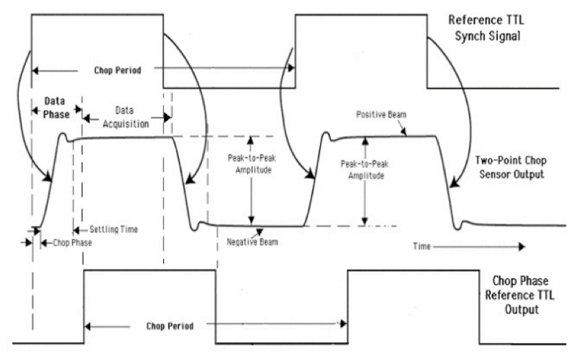
Fig. 138 Chop Phase Reference for Two-Point Chop#

Telescope astrometry#

MCCS timestamp for following fields: coord.pos.actual.tsc_mcs_hk_pkt_timestamp. Min update 10Hz.
- RA: (double64) Actual RA (hours) in J2000.0. Interpolated from MCCS: coord.pos.actual.ra. (TUNITn = ‘hours’). Possibly improved precision from incorporating ta_state.ra_rate (TBD).
- DEC: (double64) Actual DEC (degrees) in J2000.0. Interpolated from MCCS: coord.pos.actual.dec. (TUNITn = ‘degrees’) Possibly improved precision from incorporating ta_state.dec_rate (TBD).
- AZ: (double64) Actual Azimuth (degrees). Interpolated from MCCS: coord.pos.actual.azim. (TUNITn = ‘degrees’)
- EL: (double64) Actual Elevation (degrees). Interpolated from MCCS: coord.pos.actual.alt. (TUNITn = ‘degrees’)
MCCS timestamp for “desired” az/el quantities: coord.pos.desired.tsc_mcs_hk_pkt_timestamp
- AZ_Error: (double64) Azimuthal position error. Interpolated raw (unprojected) difference actual and desired azimuths (arcsec). Can be used check whether telescope is settled at the desired position. (TUNITn = ‘arcsec’) MCCS: AZ_error = 3600.0 * (coord.pos.actual.azim -coord.pos.desired.azim).
- EL_Error: (double64) Elevation position error. Interpolated difference between actual and desired elevations (arcsec). Can be used check whether telescope is settled at the desired position. (TUNITn = ‘arcsec’) MCCS: EL_error = 3600.0 * (coord.pos.actual.alt -coord.pos.desired.alt)
MCCS timestamp: coord.pos.sibs.tsc_mcs_hk_pkt_timestamp. Min update 10Hz
- SIBS_VPA: (double64) Instrument Vertical Position Angle (degrees). It is the instrument’s ‘up’ direction measured East of North. Can be used to convert focal plane offsets (e.g. pixel positions) to RA/DEC offsets relative to tracking center without having to worry about Nasmyth rotation (by EL) and Parallactic Angle. MCCS: Interpolated from coord.pos.sibs.vpa. (TUNITn = ‘degrees’).
MCCS timestamp: coord.pos.chop_ref.tsc_mcs_hk_pkt_timestamp. Update rate believed to be 10 Hz
- Chop_VPA: (double64) The Vertical Position Angle of the chopper system (degrees). It is the chopper S axis measured East of North. Can be used to convert between chopper R,S offsets and equatorial directly. MCCS: coord.pos.chop_ref.vpa. (TUNITn = ‘degrees’).
MCCS timestamp: das.gps_1_10hz.pkt_timestamp. Min update 2Hz
- LON:(double64) Geodetic longitude (degrees). Interpolated from MCCS:das.gps_1_10hz.gps_lon . (TUNITn = ‘degrees’).
- LAT: (double64) Geodetic latitude (degrees). Interpolated from MCCS:das.gps_1_10hz.gps_lat . (TUNITn = ‘degrees’)
MCCS timestamp: coord.lst.mcstime.
- LST: (double64) Local sidereal time (hours). Interpolated from MCCS: coord.lst. (TUNITn = ‘hours’).
MCCS timestamp: coord.pos.tabs.tsc_mcs_hk_pkt_timestamp). Min update 10Hz
- LOS: (double64) Line-of-sight angle (degrees). MCCS: coord.pos.tabs.los. (TUNITn = ‘degrees’).
- XEL: (double64) Cross Elevation (degrees). MCCS: coord.pos.tabs.xel. (TUNITn = ‘degrees’)
- TABS_VPA: (double64) The telescope’s Vertical Position Angle (degrees). It is the telescope vertical axis measured East of North. Can be used to convert between telescope’s native offsets and equatorial directly. MCCS: coord.pos.tabs.vpa. (TUNITn = ‘degrees’).
MCCS timestamp: das.ic1080_10hz.pitch_sampletime). Min update 2Hz
- Pitch: (float32) Aircraft pitch angle (degrees). MCCS: das.ic1080_10hz.pitch (TUNITn = ‘degrees’).
MCCS timestamp: das.ic1080_5hz.roll_sampletime). Min update 2Hz, should get 5Hz update.
- Roll: (float32) Aircraft roll angle (degrees). MCCS: das.ic1080_5hz (TUNITn = ‘degrees’).
NonSiderealRA: (double64) RA (hours) in J2000.0 of non-sidereal target. NaNs if target is not non-sidereal. Interpolated from MCCS: coord.pos.<target>.ra. (TUNITn = ‘hours’).
NonSiderealDec: (double64) Actual DEC (degrees) in J2000.0 of non-sidereal target. NaNs if target is not non-sidereal. Interpolated from MCCS: coord.pos.<target>.dec. (TUNITn = ‘degrees’)
Flag: (int32) Status flag: 0=observing, 1=LOS rewinding, 2=Running IV curve 3= between scans (TUNITn = ‘flag’).

Chop / Nod#

MCCS timestamp: coord.lst.mcstime
- NOD_OFF: (double64) Commanded nod offset (arcsec). Calculated using MCCS:nod.amplitude and nod.current. (TUNITn = ‘arcsec’) E.g. if nod.position is ‘a’ and ‘b’, then Nod_Offset = nod.amplitude for ‘a’, and Nod_Offset = -nod.amplitude for ‘b’, and NaN otherwise.

Environment / Weather#

PWV: (double64) Precipitable water-vapor level at zenith (microns). May be inaccurate and flaky, but does not hurt to record it. Nearest (or interpolated) value from MCCS: wvm_if.wvmdata.water-vapor. (TUNITn = ‘um’)

Notes#

nod/nodpol pipelines: The following columns are required for demodulation in the nod and nodpol pipelines: R array, T array, Chop Offset, Nod Offset, HWP Angle, Azimuth, Azimuth Error, Elevation, Elevation Error, Parallactic Angle. Any additional columns will be carried along and averaged over each chop cycle. The demodulated files have the same format as the raw files except that the columns R array and T array contain demodulated values. All other columns will contain values averaged over each chop cycle.