Kernel Resampling

The kernel resampler can take a set of irregular or regular data points, and interpolate them onto given coordinates through convolution with an irregular or regular kernel in N-dimensions. The base algorithm is very similar to the ResamplePolynomial class in that fits are processed in blocks according to overlaps between the sample space and fitting space. However, rather than defining a polynomial for interpolation, a spline is used to represent the given kernel and used to produce a convolution of that kernel and all samples within the range, centered at each fit coordinate.

Splines are represented and evaluated using the Spline class. Please see Splines (sofia_redux.toolkit.resampling.splines) for further details. Here, irregular refers to a set of arbitrary coordinates, while regular implies that the coordinates and values of the samples or kernel exist on a regularly spaced grid.

Use Cases

The main use case for the KernelResampler is to perform convolutions when either the sample space or kernel consists of irregular coordinates, or a smooth continuous function should be used to represent a noisy kernel. For a more standard convolution involving both regular sample space and a regular kernel, it is much faster to use standard ND convolution algorithms such as scipy.ndimage.convolve(), or the more robust sofia_redux.toolkit.convolve.kernel.KernelConvolve class.

Caveats

1. By default, an attempt will be made to fit any kernel exactly (smoothing=0). While this is suitable for most regular kernels, it may necessary to increase smoothing for irregular kernels to achieve a valid spline fit. Invalid spline fits result in a runtime error which may also provide information on how to produce a valid fit.

2. Convolution is generally of the form:

   \begin{eqnarray} f(x) = \frac{\sum_{\Omega}{d k}} {\sum_{\Omega}{k}} \end{eqnarray}

where \(\Omega\) is the window centered around \(x\), \(k\) is the kernel, and \(d\) are the data samples in the window. This is not always suitable in cases where the kernel contains negative values and may result in misleading or unexpected output results. In this case, the solution may be changed to:

\begin{eqnarray} f(x) = \frac{\sum_{\Omega}{d k}} {\sum_{\Omega}{|k|}} \end{eqnarray}

by setting absolute_weights=True during call(). By default, absolute_weights will be set to True if the kernel contains negative values and False otherwise. Note that absolute_weights will also be applied to any output weights if requested by the user.

3. The resampler naturally normalizes the kernel during convolution. If this is not desirable, the normalization can be removed by setting normalize=False during call().

Examples

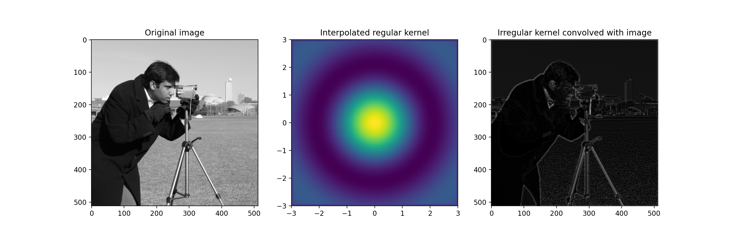
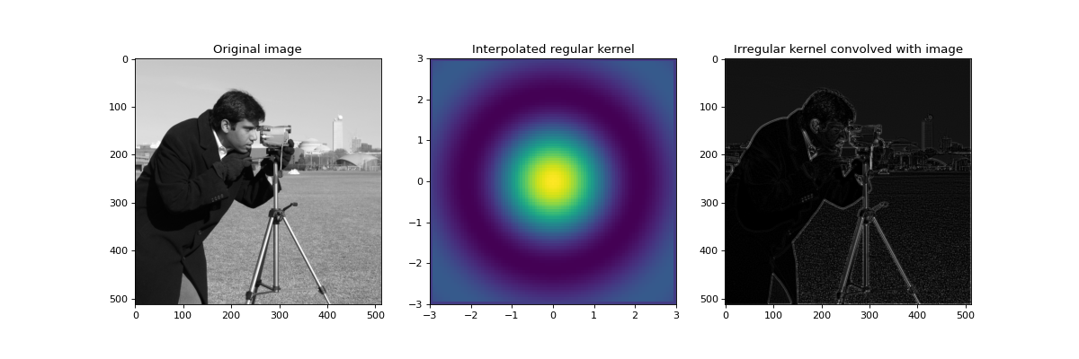
In the following example, we shall convolve an image with an irregular kernel which is effective at detecting edges. Firstly we plot a reconstructed regular kernel from the irregular input and then apply it to a regular image. Note that the kernel contains negative values so standard convolution may result in misleading values if normalization factor is not taken as the sum of absolute kernel values. This is done automatically if negative values are detected in the kernel and the absolute_weight parameter is not explicitly set by the user. Also note that the smoothing factor has been set to a small non-zero value in order to effectively fit a spline, as an exact fit may not always be possible with irregular coordinates.

import numpy as np
import matplotlib.pyplot as plt
import imageio
from sofia_redux.toolkit.resampling.resample_kernel import ResampleKernel

def mexican_hat(x, y, period=1):
    r = np.sqrt(x ** 2 + y ** 2 + np.finfo(float).eps)
    rs = r * 2 * np.pi / period
    result = np.sin(rs) / rs
    return result

# Create a set of random kernel coordinates and values
rand = np.random.RandomState(0)
width = 6
w2 = width / 2

kx = width * (rand.random(1000) - 0.5)
ky = width * (rand.random(1000) - 0.5)
kernel = mexican_hat(kx, ky, period=w2)
kernel_offsets = np.stack([kx, ky])

# First create a representation of the kernel on a grid by convolving
# with a delta function.
xx, yy = np.meshgrid(np.linspace(-w2, w2, 101), np.linspace(-w2, w2, 101))
cc = np.stack([xx.ravel(), yy.ravel()])
delta = np.zeros_like(xx)
delta[50, 50] = 1

resampler = ResampleKernel(cc, delta.ravel(), kernel, degrees=3,
                           smoothing=1e-5, kernel_offsets=kernel_offsets)

regular_kernel = resampler(cc, jobs=-1, normalize=False).reshape(
    delta.shape)

# Now show an example of edge detection using the irregular kernel
image = imageio.imread('imageio:camera.png').astype(float)
image -= image.min()
image /= image.max()

ny, nx = image.shape
iy, ix = np.mgrid[:ny, :nx]
coordinates = np.stack([ix.ravel(), iy.ravel()])
data = image.ravel()

resampler = ResampleKernel(coordinates, data, kernel, degrees=3,
                           smoothing=1e-3, kernel_offsets=kernel_offsets)
edges = abs(resampler(coordinates, jobs=-1, normalize=False)).reshape(
    image.shape)

fig, ((ax1, ax2, ax3)) = plt.subplots(1, 3, figsize=(15, 5))
ax1.imshow(image, cmap='gray')
ax1.set_title('Original image')
ax2.imshow(regular_kernel, interpolation='none', extent=[-w2, w2, -w2, w2])
ax2.set_title('Interpolated regular kernel')
ax3.imshow(edges, cmap='gray')
ax3.set_title('Irregular kernel convolved with image')

(Source code, png, hires.png, pdf)

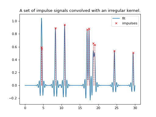
The next example shows the usage of the kernel resampler on both irregular data and an irregular kernel.

import numpy as np
import matplotlib.pyplot as plt
from sofia_redux.toolkit.resampling.resample_kernel import ResampleKernel

# Create an irregular kernel
rand = np.random.RandomState(2)
width = 4
x_range = 30
n_impulse = 10
n_kernel = 1000
n_samples = 1000

x = width * (rand.random(n_kernel) - 0.5)
kernel = np.sinc(x * 4) * np.exp(-(x ** 2))

# Add random impulses
impulse_locations = rand.random(n_samples) * x_range
impulses = np.zeros(n_samples)
impulses[:n_impulse] = 1 - 0.5 * rand.random(n_impulse)

resampler = ResampleKernel(impulse_locations, impulses, kernel,
                           kernel_offsets=x[None], smoothing=1e-6)

x_out = np.linspace(0, x_range, 500)
fit = resampler(x_out, normalize=False)

plt.plot(x_out, fit, label='fit')
plt.vlines(impulse_locations[:n_impulse], 0, impulses[:n_impulse],
           linestyles='dashed', colors='r', linewidth=1)
plt.plot(impulse_locations[:n_impulse], impulses[:n_impulse], 'x',
         color='r', label='impulses')
plt.legend()
plt.title('A set of impulse signals convolved with an irregular kernel.')

(Source code, png, hires.png, pdf)