sofia_redux.toolkit.interpolate.interpolate contains algorithms allowing interpolation from a regular grid in N-dimensions along with error propagation, and 1-dimensional functions for spline, sinc, and domain interpolation. Many algorithms were inspired by, or expanded upon, base IDL functions that were extremely useful, but never fully implemented in the major Python libraries.

The Interpolate class allows interpolation of values from those supplied on a regular grid. Interpolants are derived from N-dimensional grids of samples, optionally supplied with 1-dimensional ordinates for each dimension. NaNs may be ignored or propagated as desired.

Interpolation Schemes

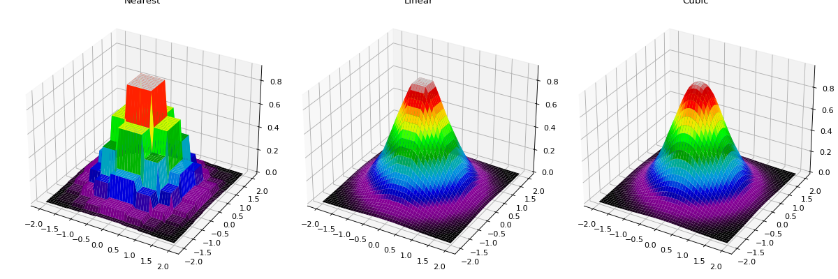
Currently there are three interpolation schemes: linear, nearest neighbor and cubic. Linear interpolation is achieved by taking the weighted average of the two neighboring points for each interpolant over each dimension using the following weights:

\begin{eqnarray} w_0 & = \frac{x - x_0}{x_1 - x_0} \\ w_1 & = \frac{x_1 - x}{x_1 - x_0} \end{eqnarray}

Cubic interpolation is achieved by applying a convolution operator across each dimension using the following kernel:

\[\begin{split}W(x) = \begin{cases} (a+2)|x|^3-(a+3)|x|^2+1 & \text{for } |x| \leq 1, \\ a|x|^3-5a|x|^2+8a|x|-4a & \text{for } 1 < |x| < 2, \\ 0 & \text{otherwise}, \end{cases}\end{split}\]

where \(a\) is usually set to -0.5 (default) or -0.75. Setting \(a = -0.5\) produces third-order convergence with respect to the sampling interval of the original grid. Note that accurate interpolation requires that each interpolant is bounded by samples in each dimension such that there are two samples to the “left” and “right”, i.e., 4 samples per dimension.

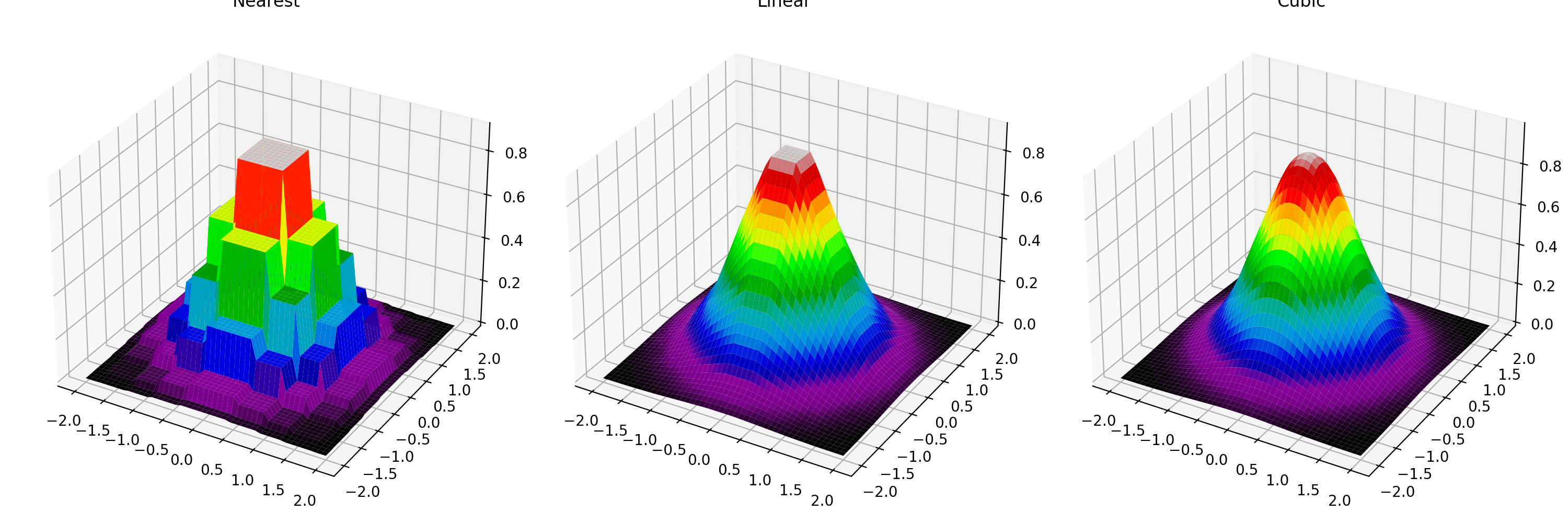
The following plot shows nearest neighbor, linear, and cubic interpolation (left to right) interpolating from a coarse regular grid to a finer resolution.

import numpy as np
import matplotlib.pyplot as plt
from mpl_toolkits.mplot3d import Axes3D
from sofia_redux.toolkit.interpolate.interpolate import Interpolate

x = np.linspace(-2, 2, 10)
y = x.copy()
xx, yy = np.meshgrid(x, y)
zz = np.exp(-((xx ** 2) + (yy ** 2)))

fig, ax = plt.subplots(nrows=1, ncols=3, figsize=(15, 5),
                       subplot_kw={'projection': '3d'})
fig.tight_layout()
xout = np.linspace(-2, 2, 50)
yout = xout.copy()
xxout, yyout = np.meshgrid(xout, yout)
cmap = 'nipy_spectral'

interpolator = Interpolate(x, y, zz, method='nearest')
z_nearest = interpolator(xxout, yyout, mode='nearest')
ax[0].set_title("Nearest")
ax[0].plot_surface(xxout, yyout, z_nearest, cmap=cmap,
                   rstride=1, cstride=1, linewidth=0)

interpolator = Interpolate(x, y, zz, method='linear')
z_linear = interpolator(xxout, yyout, mode='nearest')
ax[1].set_title("Linear")
ax[1].plot_surface(xxout, yyout, z_linear, cmap=cmap,
                   rstride=1, cstride=1, linewidth=0)

interpolator = Interpolate(x, y, zz, method='cubic')
z_cubic = interpolator(xxout, yyout, mode='nearest')
ax[2].set_title("Cubic")
ax[2].plot_surface(xxout, yyout, z_cubic, cmap=cmap,
                   rstride=1, cstride=1, linewidth=0)

(Source code, png, hires.png, pdf)

Edge effects

Accurate interpolation requires 4 samples for cubic interpolation and 2 samples for linear interpolation bounding each interpolant per dimension. This requirement cannot be met for interpolants close to the edge of the grid, so in these cases, the grid is effectively padded with values to allow an approximation to be calculated. The “mode” keyword determines the method by which this is accomplished. Available methods are:

Mode	Left pad	Samples	Right pad
nearest	1 1 1 1	1 2 3 4	4 4 4 4
reflect	4 3 2 1	1 2 3 4	4 3 2 1
mirror	4 3 2	1 2 3 4	3 2 1
wrap	1 2 3 4	1 2 3 4	1 2 3 4
constant	x x x x	1 2 3 4	x x x x

Where numbers represent sample value indices in a single dimension and x indicates a user supplied value (cval).

import numpy as np
import matplotlib.pyplot as plt
from sofia_redux.toolkit.interpolate import Interpolate

y = np.arange(10).astype(float)
x = np.arange(10).astype(float)
x1 = np.linspace(-1, 2, 51)

interpolator = Interpolate(x, y, method='cubic', mode='nearest')
y_nearest = interpolator(x1)

interpolator = Interpolate(x, y, method='cubic', cval=1)
y_constant = interpolator(x1)

interpolator = Interpolate(x, y, method='cubic', mode='wrap')
y_wrap = interpolator(x1)

plt.figure(figsize=(5, 5))
plt.xlim(-1, 2)
plt.ylim(-1, 2)
plt.xlabel('X')
plt.ylabel('Y')
plt.title("Edge Modes")
plt.plot(x, y, 's', color='k', linewidth=10, label='samples')
plt.plot(x1, y_nearest, label='nearest')
plt.plot(x1, y_constant, label='constant=1')
plt.plot(x1, y_wrap, label='wrap')
plt.legend()

(Source code, png, hires.png, pdf)

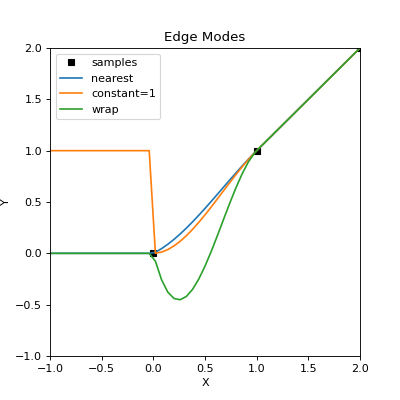
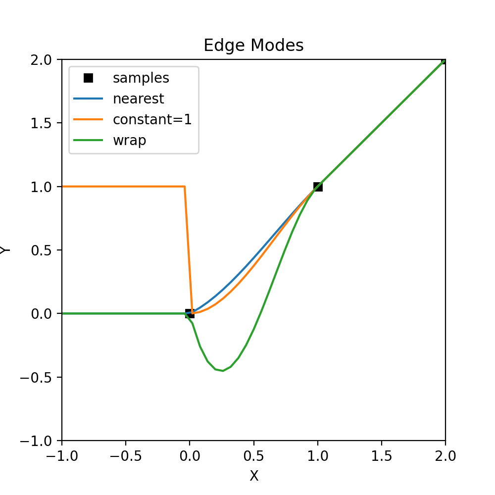
The above plot gives a basic idea on how edge effects can manifest and the influence of the edge “mode”. Cubic interpolation is used as it is most sensitive to any edge effects. The edge shown is at \(x < 0\), outside the sample domain, which clearly has an affect on interpolants where \(x < 1\). Here, the “nearest” edge mode best represents the actual samples, while the “wrap” mode provides a poor fit as missing values were replaced with those from the other end of the sample array.

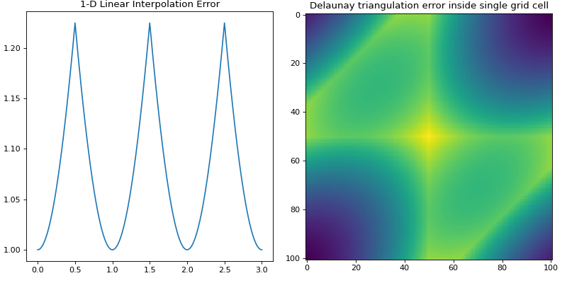
Linear Interpolation Error Propagation

If using linear interpolation in 1-dimension or Delaunay triangulation in N-dimensions, errors may be propagated using the function interp_error() in N-dimensions.

from sofia_redux.toolkit.interpolate import interp_error
import numpy as np
import matplotlib.pyplot as plt

x = np.arange(10)
error = np.ones(10)
points_out = np.linspace(0, 3, 301)
i_error_1d = interp_error(x, error, points_out)

fig, ax = plt.subplots(nrows=1, ncols=2, figsize=(10, 5))
fig.tight_layout()

ax[0].plot(points_out, i_error_1d)
ax[0].set_title("1-D Linear Interpolation Error")

y, x = np.mgrid[:4, :4]
error = np.full(x.size, 1.0)
points = np.stack((x.ravel(), y.ravel())).T
xg = np.linspace(2.1, 2.9, 101)
points_out = np.array([x.ravel() for x in np.meshgrid(xg, xg)]).T
i_error = interp_error(points, error, points_out)
ax[1].imshow(i_error.reshape((101, 101)))
ax[1].set_title("Delaunay triangulation error inside single grid cell")

(Source code, png, hires.png, pdf)

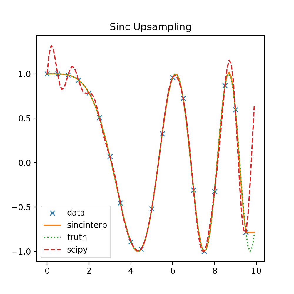
Sinc Interpolation

1-dimensional sinc interpolation is available using the sincinterp() function. The actual function uses modified sinc interpolation such that

\begin{eqnarray} y(t) & = & \sum_{i = i_{t} - N/2}^{i_{t} + N/2}{ y_{i} . sinc(x(t_{i})) . exp \left\{ \left( \frac{x(t_{i})}{\alpha} \right)^{2} \right\} } \\ i_{t} & = & max(i \, | \, x_{i} \leq x(t)) \\ x(t_{i}) & = & \frac{x(t) - x_{i_{t}}}{x_{i_{t} + 1} - x_{i_{t}}} + i \\ \end{eqnarray}

where \(\alpha\) is the dampening factor (default = 3.25) and may be disabled by setting \(\alpha=0\). Note that the sampling interval is determined by the kernel width \(N\) (default = 21) and is dependant on the distribution of the samples themselves, rather than being explicitly set by the user. This modified version of the function allows for better handling of non-periodic band-limited functions, irregular data, and NaN handling.

from sofia_redux.toolkit.interpolate import sincinterp
from scipy import signal
import numpy as np

x = np.linspace(0, 10, 20, endpoint=False)
y = np.cos(-x ** 2 / 6.0)
xout = np.linspace(0, 10, 100, endpoint=False)
yout = sincinterp(x, y, xout)
truth = np.cos(-xout ** 2 / 6)
scipy_try = signal.resample(y, 100)
plt.figure(figsize=(5, 5))
plt.plot(x, y, 'x', xout, yout, '-',
         xout, truth, ':', xout, scipy_try,'--')
plt.legend(['data', 'sincinterp', 'truth', 'scipy'],
           loc='lower left')
plt.title("Sinc Upsampling")

(Source code, png, hires.png, pdf)

The above plot shows a comparison of sincinterp() with scipy.signal.resample(). sincinterp() provides a very close fit to the actual truth, while the FFT sinc interpolation method used by scipy.signal.resample() shows an obvious deviation due to the assumption of a periodic function.

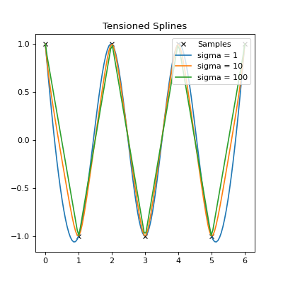
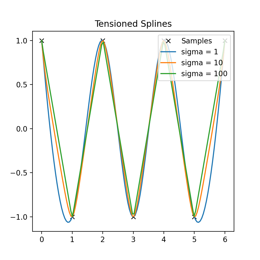
Tensioned Spline Interpolation

The spline() function performs tensioned cubic spline interpolation, recreating the functionality of the IDL spline function.

from sofia_redux.toolkit.interpolate import spline
import numpy as np
import matplotlib.pyplot as plt

x = np.arange(7).astype(float)
y = (-1) ** x

tensions = [1, 10, 100]
xout = np.linspace(x.min(), x.max(), np.ptp(x.astype(int) * 20))
fits = np.zeros((len(tensions), xout.size))
for i, sigma in enumerate(tensions):
    fits[i] = spline(x, y, xout, sigma=sigma)

plt.figure(figsize=(5, 5))
plt.plot(x, y, 'x', color='k')
for i in range(len(tensions)):
    plt.plot(xout, fits[i])
plt.title("Tensioned Splines")
legend = ['Samples']
legend += ['sigma = %s' % tensions[i] for i in range(len(tensions))]
plt.legend(legend, loc='upper right')

(Source code, png, hires.png, pdf)

The above plot shows the effect of tension (sigma) on the spline fit. For low tension, it is effectively a cubic spline fit. For higher tensions, the fit is closer to polynomial interpolation.

Domain Interpolation

tabinv() is used to find the effective index of a function value in an ordered 1-dimensional vector using linear interpolation. The function in question should be monotonically increasing or decreasing.

from sofia_redux.toolkit.interpolate import tabinv
x = [np.nan, np.nan, 1, 2, np.nan, 3, 4, 5]
assert tabinv(x, 1.5) == 2.5
assert tabinv(x, 3.25) == 5.25

A binary search is used to find the values x[i] and x[i+1] where:

\[i_{t} = \frac{x(t) - x_{i}}{x_{i + 1} - x_{i}} + i\]